本文主要聚焦在MySQL最新版本官方的源码上,重点分析了官方的重构在多阶段和各阶段结构上的变化和联系,更多是为了了解一个全新的MySQL的发展。
背景与架构
之前对MySQL的理解是建立在5.6和5.7版本之上,更多的是对比PostgreSQL或者传统数据库。然而从MySQL 8.0开始,通过持续每三个月的迭代和重构工作,使得MySQL Server层的整体架构有了质的飞越。
本文基于MySQL 8.0.25源码进行分析和总结,介绍MySQL的最新架构。其中MySQL Server层指的是MySQL的优化器、执行器部分。
架构图如下所示: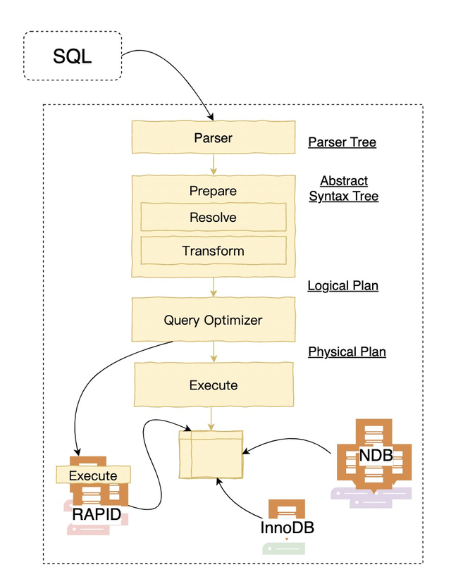 最新的MySQL的分层架构和其他数据库并没有太大的区别,而MySQL现在更多的是加强InnoDB、NDB集群和RAPID(HeatWave clusters)内存集群架构的演进。本文更偏向于从优化器、执行器的流程角度来演进。
最新的MySQL的分层架构和其他数据库并没有太大的区别,而MySQL现在更多的是加强InnoDB、NDB集群和RAPID(HeatWave clusters)内存集群架构的演进。本文更偏向于从优化器、执行器的流程角度来演进。
MySQL 解析器Parser
官方MySQL 8.0使用Bison进行了重写,生成Parser Tree,同时Parser Tree会通过contextualize函数生成MySQL抽象语法树(Abstract
Syntax Tree)。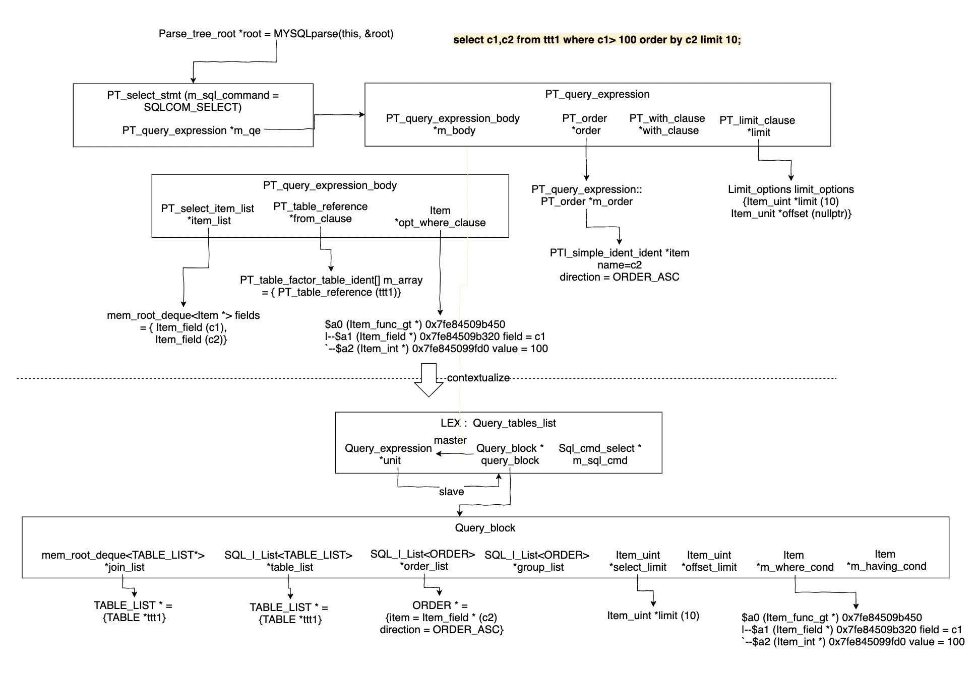
MySQL抽象语法树和其他数据库有些不同,是由比较让人拗口的
SELECT_LEX_UNIT/SELECT_LEX类交替构成的,然而这两个结构在最新的版本中已经重命名成标准的SELECT_LEX -> Query_block和SELECT_LEX_UNIT -> Query_expression。
说明
- Query_block:表示查询块。
- Query_expression:表示包含多个查询块的查询表达式,包括
UNION AND/OR的查询块(例如,SELECT * FROM t1 union SELECT * FROM t2)或者有多Level的ORDER BY/LIMIT(例如,SELECT * FROM t1 ORDER BY a LIMIT 10)ORDER BY b LIMIT 5。
以下示例是一个复杂的嵌套查询: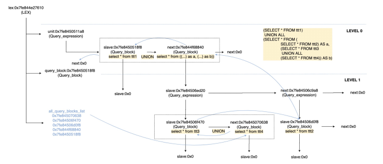 经过解析和转换后的语法树仍然建立在
(SELECT *
   FROM ttt1)
UNION ALL
  (SELECT *
   FROM
     (SELECT *
      FROM ttt2) AS a,
     (SELECT *
      FROM ttt3
      UNION ALL SELECT *
FROM ttt4) AS b)Query_block和Query_expression的框架下,只不过有些LEVEL的query block被消除或者合并了,此处不再赘述。
MySQL prepare/rewrite阶段
接下来需要经过解析(resolve)和转换(transformation)过程(函数:Query_expression::prepare->Query_block::prepare),此过程流程如下(按功能分而非完全按照执行顺序):
- Setup and Fix
- setup_tables:Set up table leaves in the query block based on list of tables.
- resolve_placeholder_tables/merge_derived/setup_table_function/setup_materialized_derived:Resolve derived table, view or table function references in query block.
- setup_natural_join_row_types:Compute and store the row types of the top-most NATURAL/USING joins.
- setup_wild:Expand all '*' in list of expressions with the matching column references.
- setup_base_ref_items:Set query_block's base_ref_items.
- setup_fields:Check that all given fields exists and fill struct with current data.
- setup_conds:Resolve WHERE condition and join conditions.
- setup_group:Resolve and set up the GROUP BY list.
- m_having_cond->fix_fields:Setup the HAVING clause.
- resolve_rollup:Resolve items in SELECT list and ORDER BY list for rollup processing.
- resolve_rollup_item:Resolve an item (and its tree) for rollup processing by replacing items matching grouped expressions with Item_rollup_group_items and updating properties (m_nullable, PROP_ROLLUP_FIELD). Also check any GROUPING function for incorrect column.
- setup_order:Set up the ORDER BY clause.
- resolve_limits:Resolve OFFSET and LIMIT clauses.
- Window::setup_windows1:Set up windows after setup_order() and before setup_order_final().
- setup_order_final:Do final setup of ORDER BY clause, after the query block is fully resolved.
- setup_ftfuncs:Setup full-text functions after resolving HAVING.
- resolve_rollup_wfs : Replace group by field references inside window functions with references in the presence of ROLLUP.
- Transformation
- remove_redundant_subquery_clause : Permanently remove redundant parts from the query if 1) This is a subquery 2) Not normalizing a view. Removal should take place when a query involving a view is optimized, not when the view is created.
- remove_base_options:Remove SELECT_DISTINCT options from a query block if can skip distinct.
- resolve_subquery : Resolve predicate involving subquery, perform early unconditional
subquery transformations.
- Convert subquery predicate into semi-join, or
- Mark the subquery for execution using materialization, or
- Perform IN->EXISTS transformation, or
- Perform more/less ALL/ANY -> MIN/MAX rewrite
- Substitute trivial scalar-context subquery with its value
- transform_scalar_subqueries_to_join_with_derived:Transform eligible scalar subqueries to derived tables.
- flatten_subqueries:Convert semi-join subquery predicates into semi-join join nests. Convert candidate subquery predicates into semi-join join nests. This transformation is performed once in query lifetime and is irreversible.
- apply_local_transforms:
- delete_unused_merged_columns : If query block contains one or more merged derived tables/views, walk through lists of columns in select lists and remove unused columns.
- simplify_joins:Convert all outer joins to inner joins if possible
- prune_partitions:Perform partition pruning for a given table and condition.
- push_conditions_to_derived_tables:Pushing conditions down to derived tables must be done after validity checks of grouped queries done by apply_local_transforms();
- Window::eliminate_unused_objects:Eliminate unused window definitions, redundant sorts etc.
此处只列举和top_join_list相关的simple_joins函数的作用,对于Query_block中嵌套join的简化过程。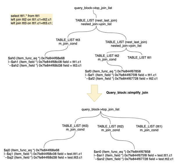
- 对比PostgreSQL。
为了更清晰的理解标准数据库的做法,此处引用了PostgreSQL的三个过程:
- Parser
如下图所示,Parser将SQL语句生成parse tree。
SELECT id, data FROM tbl_a WHERE id < 300 ORDER BY data;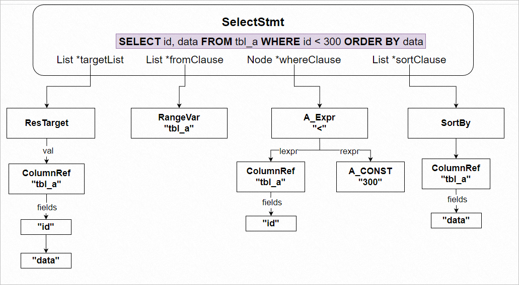
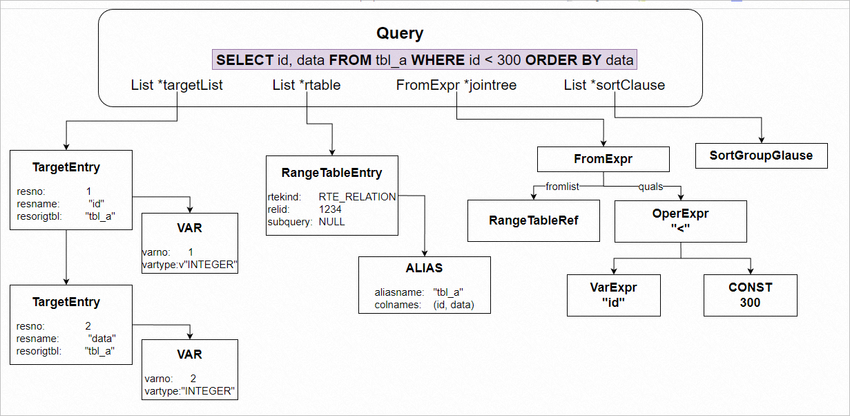
- Analyzer/Analyser
下图展示了PostgreSQL的analyzer/analyser如何将parse tree通过语义分析后生成query tree。
- Rewriter
Rewriter会根据系统中的规则将query tree进行转换改写。
下图的示例为一个包含view的query tree如何展开成新的query tree。sampledb=# CREATE VIEW employees_list sampledb-# AS SELECT e.id, e.name, d.name AS department sampledb-# FROM employees AS e, departments AS d WHERE e.department_id = d.id;sampledb=# SELECT * FROM employees_list;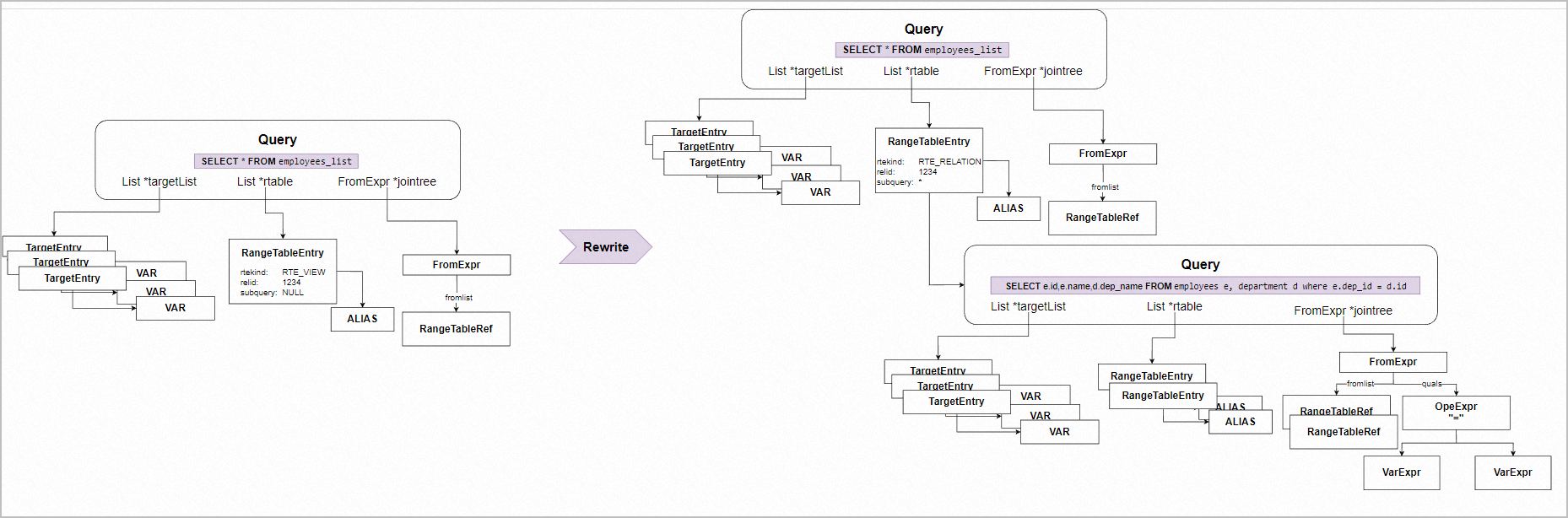
- Parser
MySQL Optimize和Planning阶段
此阶段为逻辑计划生成物理计划的过程,本文注重结构的解析,而不介绍生成的细节。
MySQL在8.0.22之前,主要依赖的结构为JOIN和QEP_TAB,JOIN是与之对应的每个Query_block,而QEP_TAB对应的每个Query_block涉及到的具体“表”的顺序、方法和执行计划。
然而在8.0.22之后,新的基于Hypergraph的优化器算法丢弃了QEP_TAB结构来表达左深树的执行计划,而直接使用HyperNode/HyperEdge的图来表示执行计划。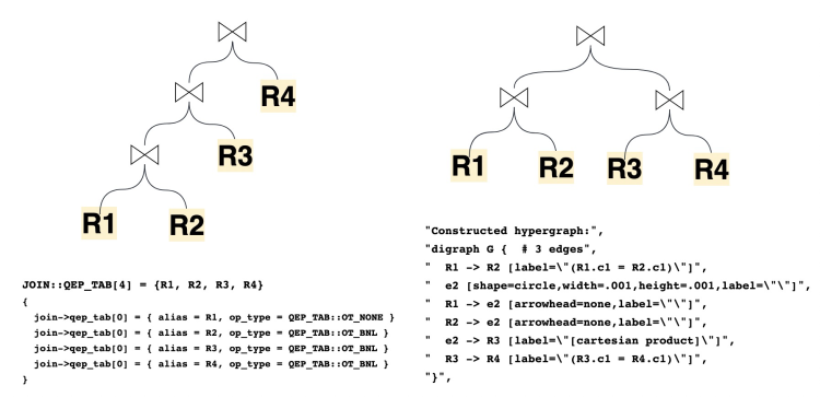 可以看到数据结构表达的left deep tree和超图结构表达的bushy tree对应的不同计划展现:
可以看到数据结构表达的left deep tree和超图结构表达的bushy tree对应的不同计划展现:| -> Inner hash join (no condition) (cost=1.40 rows=1)
-> Table scan on R4 (cost=0.35 rows=1)
-> Hash
-> Inner hash join (no condition) (cost=1.05 rows=1)
-> Table scan on R3 (cost=0.35 rows=1)
-> Hash
-> Inner hash join (no condition) (cost=0.70 rows=1)
-> Table scan on R2 (cost=0.35 rows=1)
-> Hash
-> Table scan on R1 (cost=0.35 rows=1)
| -> Nested loop inner join (cost=0.55..0.55 rows=0)
-> Nested loop inner join (cost=0.50..0.50 rows=0)
-> Table scan on R4 (cost=0.25..0.25 rows=1)
-> Filter: (R4.c1 = R3.c1) (cost=0.35..0.35 rows=0)
-> Table scan on R3 (cost=0.25..0.25 rows=1)
-> Nested loop inner join (cost=0.50..0.50 rows=0)
-> Table scan on R2 (cost=0.25..0.25 rows=1)
-> Filter: (R2.c1 = R1.c1) (cost=0.35..0.35 rows=0)
-> Table scan on R1 (cost=0.25..0.25 rows=1)MySQL8.0.2x为了更好的兼容两种优化器,引入了新的类AccessPath,可以认为这是MySQL为了解耦执行器和不同优化器抽象出来的Plan Tree。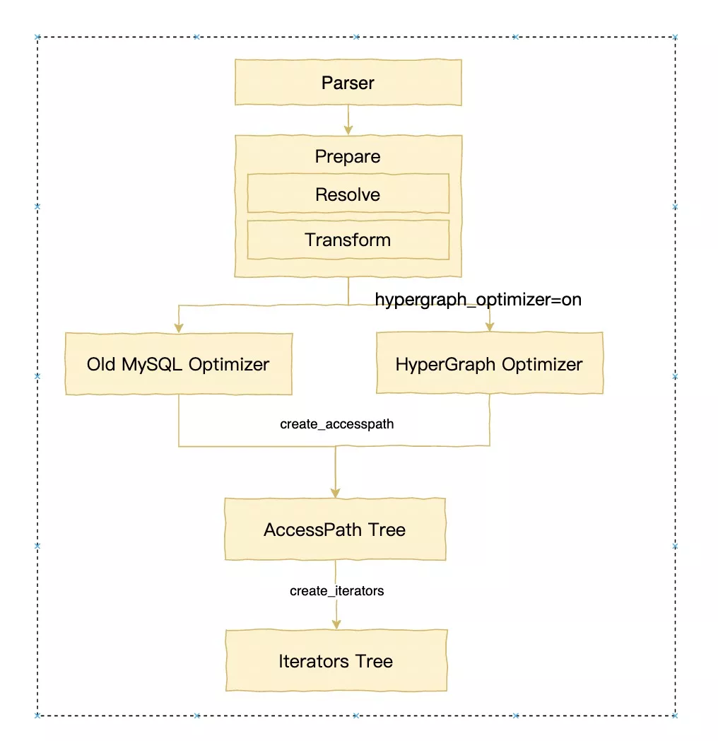
- 老优化器入口。
老优化器仍然通过JOIN::optimize将query block转换成query execution plan (QEP)。这个阶段仍然做一些逻辑的重写工作,这个阶段的转换可以理解为基于cost-based优化前做准备,详细步骤如下:
- Logical transformations
- optimize_derived : Optimize the query expression representing a derived table/view.
- optimize_cond : Equality/constant propagation.
- prune_table_partitions : Partition pruning.
- optimize_aggregated_query : COUNT(*), MIN(), MAX() constant substitution in case of implicit grouping.
- substitute_gc : ORDER BY optimization, substitute all expressions in the WHERE condition and ORDER/GROUP lists that match generated columns (GC) expressions with GC fields, if any.
- Perform cost-based optimization of table order and access path selection.
JOIN::make_join_plan() : Set up join order and initial access paths.
- Post-join order optimization.
- substitute_for_best_equal_field : Create optimal table conditions from the where clause and the join conditions.
- make_join_query_block : Inject outer-join guarding conditions.
- Adjust data access methods after determining table condition (several times).
- optimize_distinct_group_order : Optimize ORDER BY/DISTINCT.
- optimize_fts_query : Perform FULLTEXT search before all regular searches.
- remove_eq_conds : Removes const and eq items. Returns the new item, or nullptr if no condition.
- replace_index_subquery/create_access_paths_for_index_subquery : See if this subquery can be evaluated with subselect_indexsubquery_engine.
- setup_join_buffering : Check whether join cache could be used.
- Code generation
- alloc_qep(tables) : Create QEP_TAB array.
- test_skip_sort : Try to optimize away sorting/distinct.
- make_join_readinfo : Plan refinement stage: do various setup things for the executor.
- make_tmp_tables_info : Setup temporary table usage for grouping and/or sorting.
- push_to_engines : Push (parts of) the query execution down to the storage engines if they can provide faster execution of the query, or part of it.
- create_access_paths : generated ACCESS_PATH.
- Logical transformations
- 新优化器入口。
新优化器默认关闭,必须通过
set optimizer_switch="hypergraph_optimizer=on";开启。主要通过FindBestQueryPlan函数来实现,逻辑如下所示:- 判断是否属于新优化器可以支持的Query语法(CheckSupportedQuery),不支持的直接返回
ER_HYPERGRAPH_NOT_SUPPORTED_YET错误。 - 转化top_join_list为JoinHypergraph结构。由于Hypergraph是比较独立的算法层面的实现,JoinHypergraph结构用于更好的把数据库的结构包装到Hypergraph的edges和nodes的概念上。
- 通过EnumerateAllConnectedPartitions实现论文《Dynamic Programming Strikes Back》中的DPhyp算法。
- CostingReceiver类包含过去JOIN planning的主要逻辑,包括根据cost选择相应的访问路径,根据DPhyp生成的子计划进行评估,保留cost最小的子计划。
- 得到root_path后,再处理group/agg/having/sort/limit的。对于Group by操作,目前Hypergraph使用sorting first + streaming aggregation的方式。
以下示例用于说明Plan(AccessPath)和SQL的关系。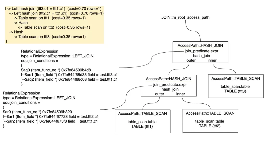 最后生成Iterator执行器框架需要的Iterator执行载体,AccessPath和Iterator是一对一的关系(Access paths are a query planning structure that correspond 1:1 to iterators)。
Query_expression::m_root_iterator = CreateIteratorFromAccessPath(......) unique_ptr_destroy_only<RowIterator> CreateIteratorFromAccessPath( THD *thd, AccessPath *path, JOIN *join, bool eligible_for_batch_mode) { ...... switch (path->type) { case AccessPath::TABLE_SCAN: { const auto ¶m = path->table_scan(); iterator = NewIterator<TableScanIterator>( thd, param.table, path->num_output_rows, examined_rows); break; } case AccessPath::INDEX_SCAN: { const auto ¶m = path->index_scan(); if (param.reverse) { iterator = NewIterator<IndexScanIterator<true>>( thd, param.table, param.idx, param.use_order, path->num_output_rows, examined_rows); } else { iterator = NewIterator<IndexScanIterator<false>>( thd, param.table, param.idx, param.use_order, path->num_output_rows, examined_rows); } break; } case AccessPath::REF: { ...... } - 判断是否属于新优化器可以支持的Query语法(CheckSupportedQuery),不支持的直接返回
- 对比PostgreSQL。
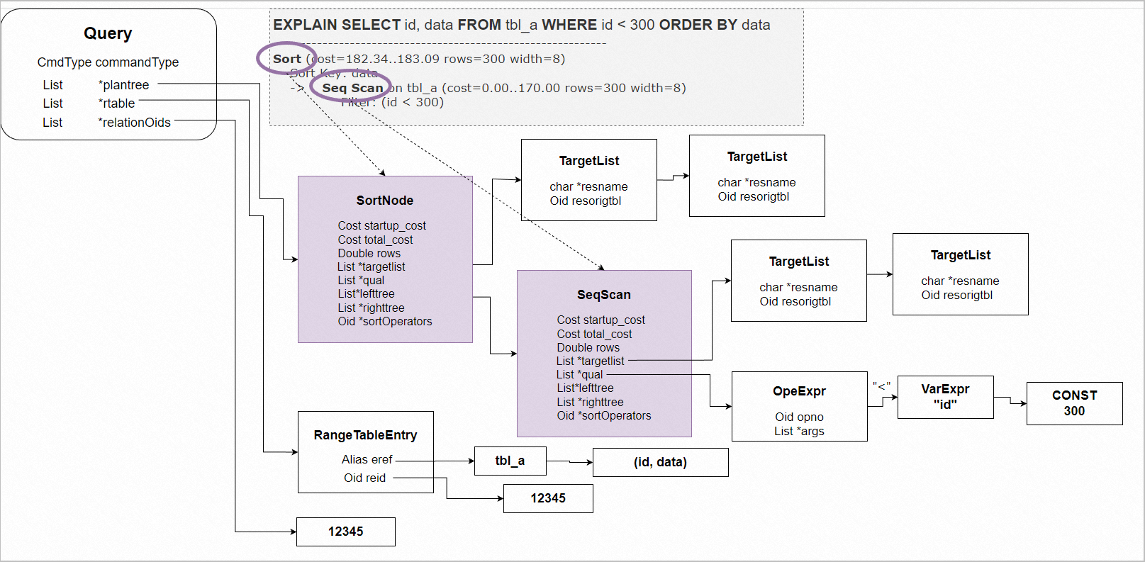
testdb=# EXPLAIN SELECT * FROM tbl_a WHERE id < 300 ORDER BY data;
                          QUERY PLAN
---------------------------------------------------------------
 Sort  (cost=182.34..183.09 rows=300 width=8)
   Sort Key: data
   ->  Seq Scan on tbl_a  (cost=0.00..170.00 rows=300 width=8)
         Filter: (id < 300)
(4 rows)