雷达数据可视化

场景简介

• 本实验介绍：jupyter notebook中运行的雷达数据可视化代码

实验室资源方式简介

进入实操前，请确保阿里云账号满足以下条件：

• 个人账号资源

  • 使用您个人的云资源进行操作，资源归属于个人。

  • 平台仅提供手册参考，不会对资源做任何操作。

• 确保已完成云工开物300元代金券领取。

• 已通过实名认证且账户余额≥100元。

本次实验将在您的账号下开通实操所需计算型实例规格族c7a，费用约为：25元（以实验时长2小时预估，具体金额取决于实验完成的时间），需要您通过阿里云云工开物学生专属300元抵扣金兑换本次实操的云资源。

如果您调整了资源规格、使用时长，或执行了本方案以外的操作，可能导致费用发生变化，请以控制台显示的实际价格和最终账单为准。

领取专属权益及创建实验资源

在开始实验之前，请先点击右侧屏幕的“进入实操”再进行后续操作

领取300元高校专属权益优惠券（若已领取请跳过）

实验步骤

• 1、服务部署

  • 点击链接，进入部署页面

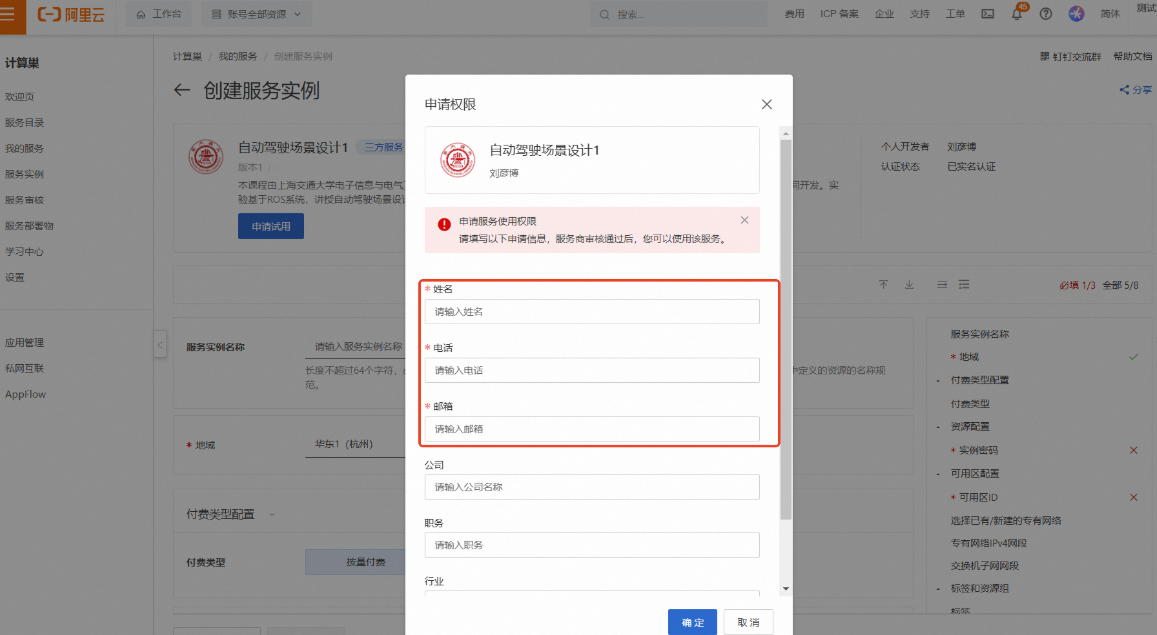
  • 按弹窗提示进行权限申请。其中【姓名】、【电话】、【邮箱】为必填项，完成填写后点击【确定】

    说明

    请填写您的学校邮箱（.edu）,便于审核

    

  • 提交申请后将提示

    

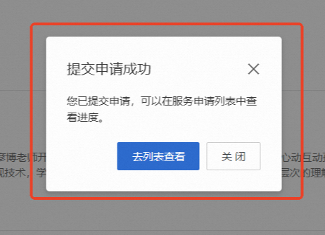
  • 当申请通过后，将会收到短信提示可以进行部署

    

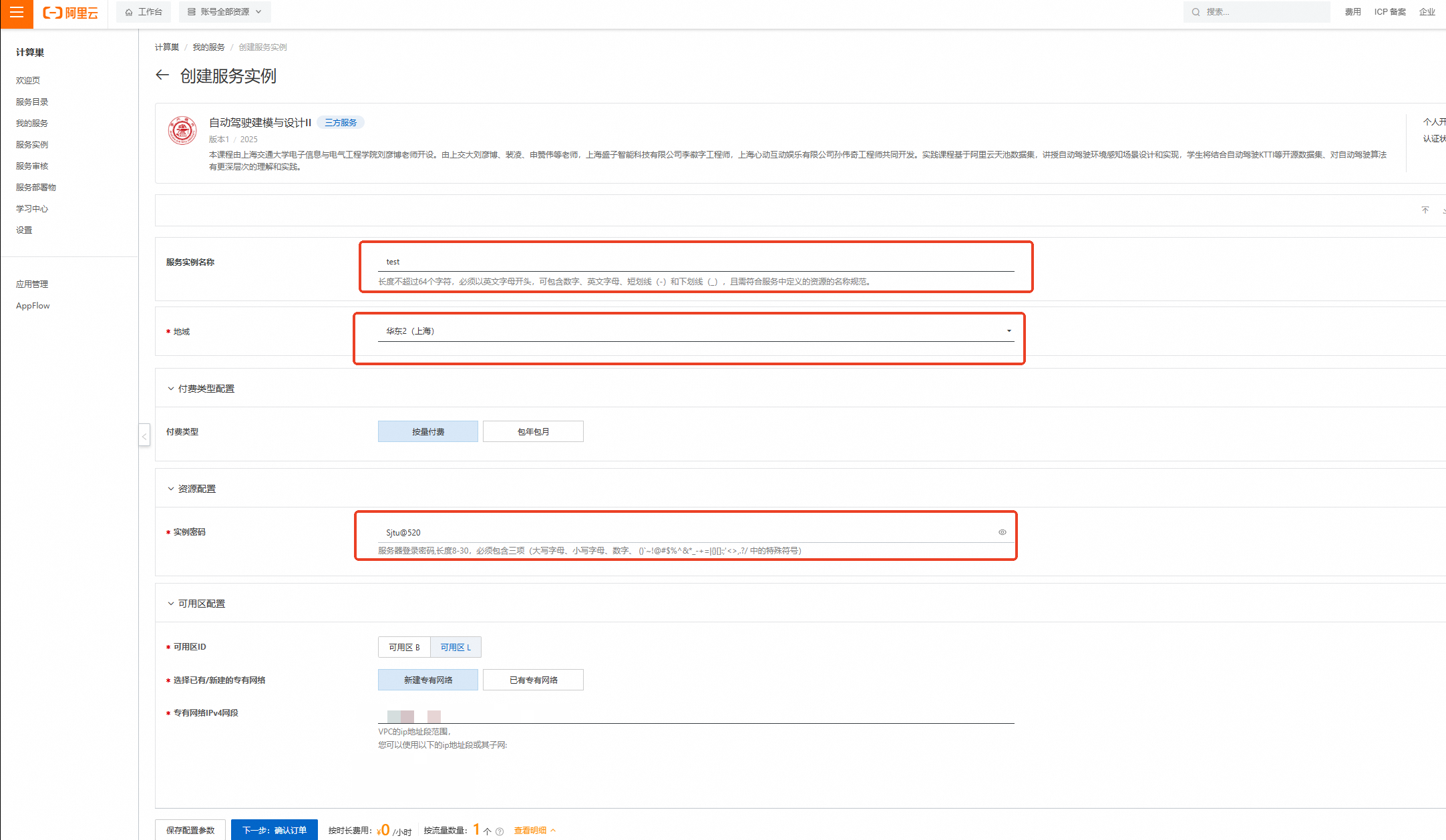
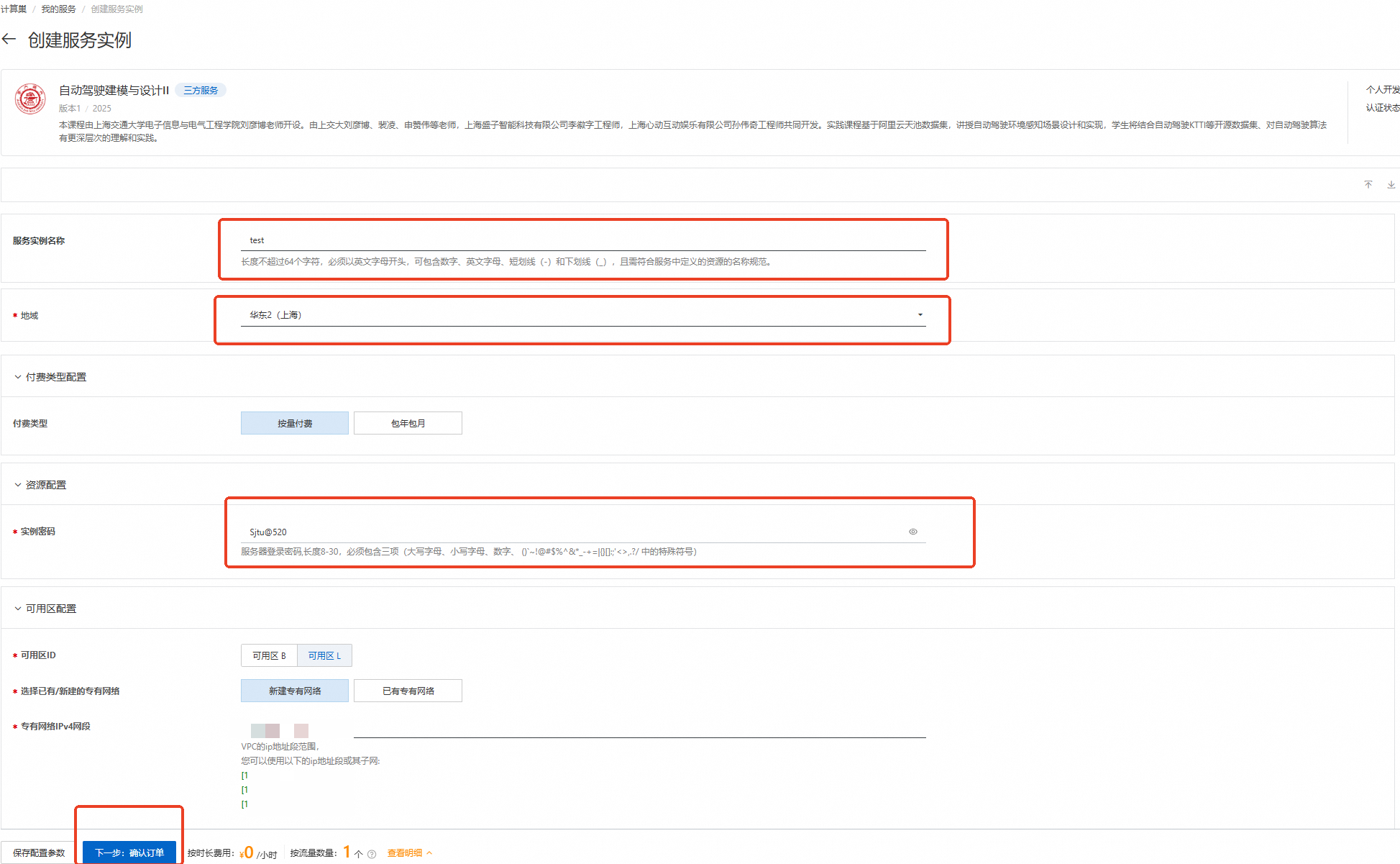
  • 刷新部署页面，按下图设置【服务实例名称】、【地域】、【实例密码】

    • 服务实例名称：test（可自定义命名）

    • 地域：华东2（上海）

    • 实例密码：Sjtu@520

      说明

      输入实例密码时请注意大小写，请记住您设置的实例名称及对应密码，后续实验过程会用到。

    

  • 完成填写后点击【下一步：确认订单】

    

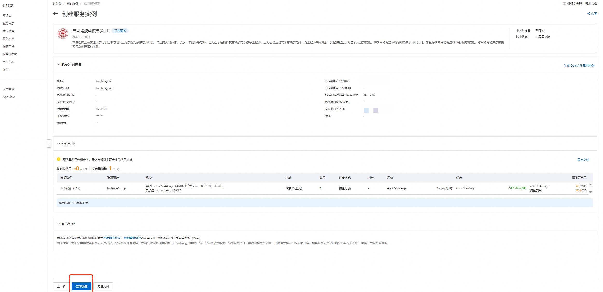
  • 核对实例信息及价格预览，无误请点击【立即创建】

    

    重要

    领取300元优惠券后，资源应为0元/小时，且会提示【您当前账户的余额充足】！若提示余额不足等，请检查是否正确领取优惠券

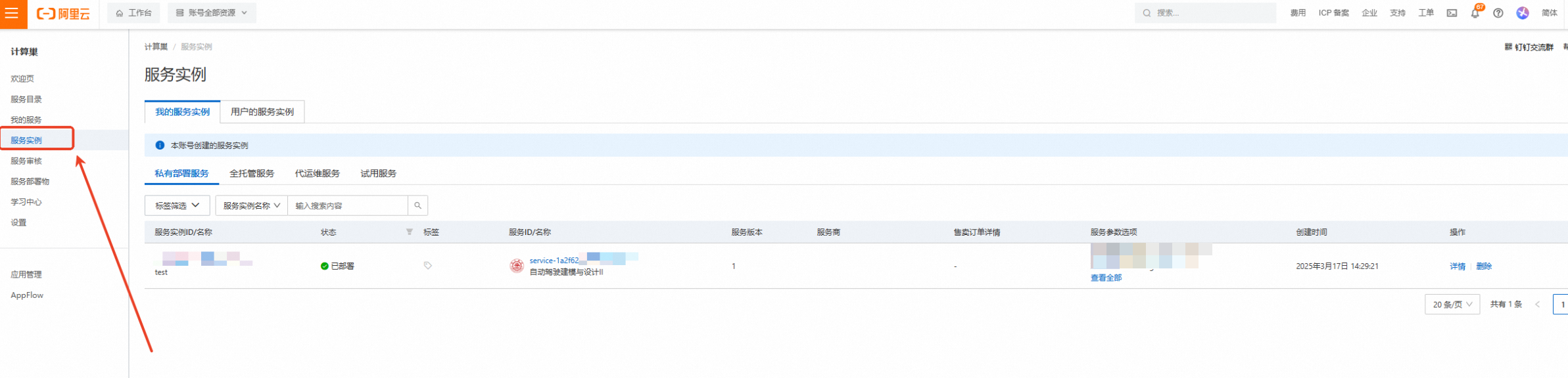
  • 创建成功，点击【去列表查看】

    

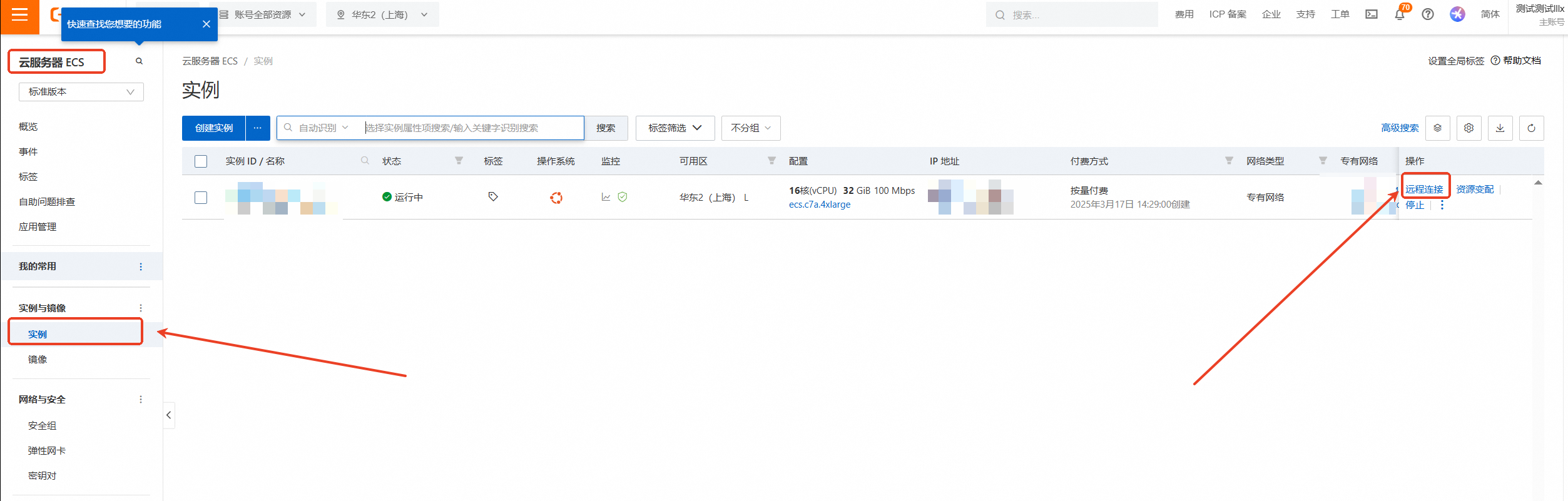
  • 查看实例，点击左侧的图标展开目录

    

    选择目录中的【云服务器ECS】

    

  • 云服务器ECS—实例—远程连接

    

  • 下拉展开更多登录方式，选择【通过VNC远程连接】

    

  • 输入实例密码：Sjtu@520（请输入您设置的密码）后回车

    

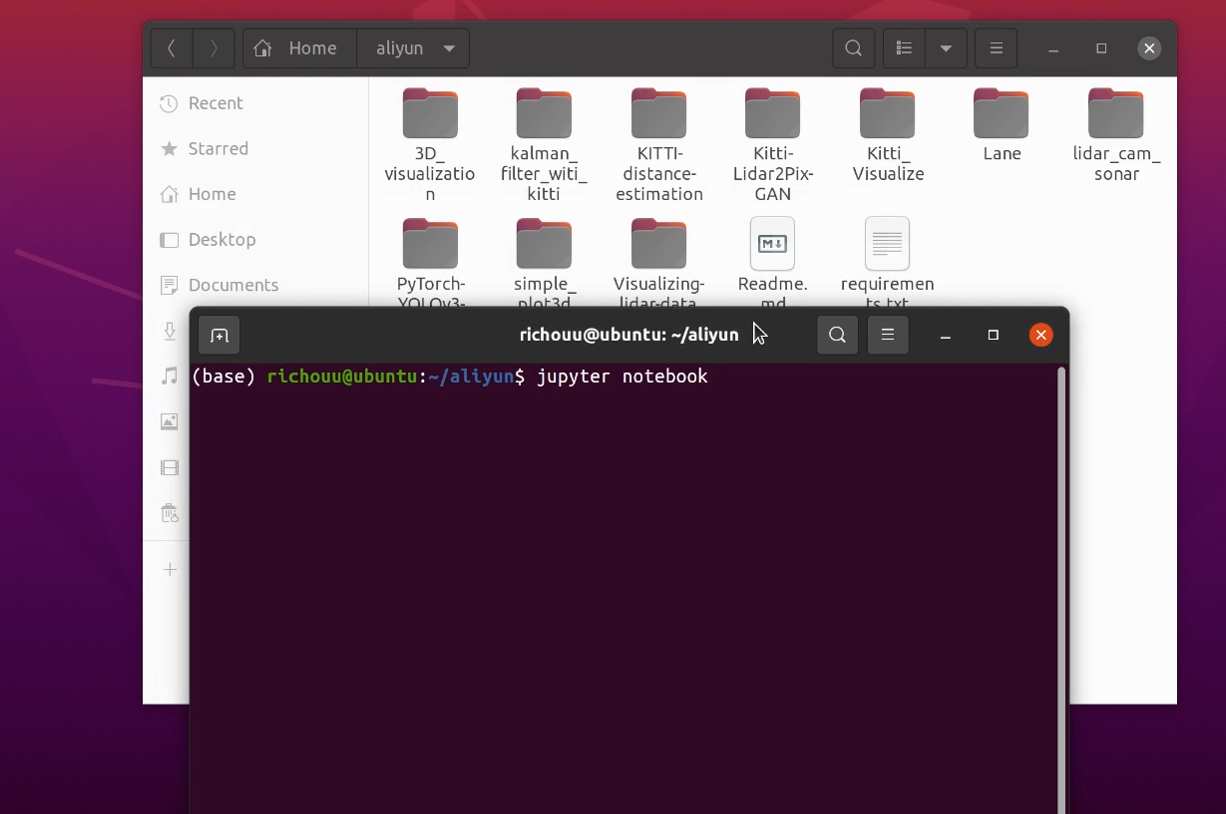
  • 进入Ubuntu20.04系统后打开aliyun文件夹，在文件夹中右键开启终端并输入 /jupyter notebook 命令，用户名前面的(base)表示此时处于anaconda的base环境中

    

• 2、打开文件并运行

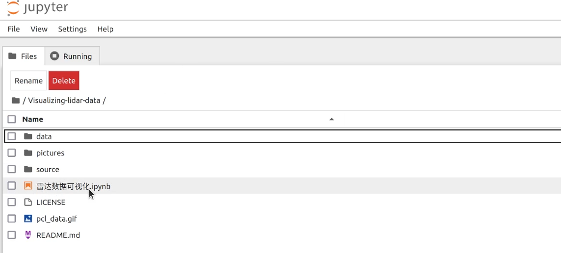
  在自动弹出的浏览器页面中选择/Visualizing-lidar-data/雷达数据可视化.ipynb并打开

  

  点击此选项可按步运行

  

• 3、读取数据集

  import numpy as np
  import pykitti
  
  basedir = '/home/ecs-user/aliyun/Visualizing-lidar-data/data'
  
  def load_dataset(date, drive, calibrated=False, frame_range=None):
      dataset = pykitti.raw(basedir, date, drive)
  
      # 加载数据
      if calibrated:
          dataset.load_calib()  # Calibration data are accessible as named tuples
  
      np.set_printoptions(precision=4, suppress=True)
      print('\nDrive: ' + str(dataset.drive))
      print('\nFrame range: ' + str(dataset.frames))
  
      if calibrated:
          print('\nIMU-to-Velodyne transformation:\n' + str(dataset.calib.T_velo_imu))
          print('\nGray stereo pair baseline [m]: ' + str(dataset.calib.b_gray))
          print('\nRGB stereo pair baseline [m]: ' + str(dataset.calib.b_rgb))
  
      return dataset

• 4、读取轨迹数据

  import sys
  sys.path.append("/home/ecs-user/aliyun/Visualizing-lidar-data/source")
  print(sys.path)
  import parseTrackletXML as xmlParser
  def load_tracklets_for_frames(n_frames, xml_path):
      tracklets = xmlParser.parseXML(xml_path)
  
      frame_tracklets = {}
      frame_tracklets_types = {}
      for i in range(n_frames):
          frame_tracklets[i] = []
          frame_tracklets_types[i] = []
  
      for i, tracklet in enumerate(tracklets):
          h, w, l = tracklet.size
          trackletBox = np.array([
              [-l / 2, -l / 2, l / 2, l / 2, -l / 2, -l / 2, l / 2, l / 2],
              [w / 2, -w / 2, -w / 2, w / 2, w / 2, -w / 2, -w / 2, w / 2],
              [0.0, 0.0, 0.0, 0.0, h, h, h, h]
          ])
          for translation, rotation, state, occlusion, truncation, amtOcclusion, amtBorders, absoluteFrameNumber in tracklet:
              if truncation not in (xmlParser.TRUNC_IN_IMAGE, xmlParser.TRUNC_TRUNCATED):
                  continue
              yaw = rotation[2]
              assert np.abs(rotation[:2]).sum() == 0, 'object rotations other than yaw given!'
              rotMat = np.array([
                  [np.cos(yaw), -np.sin(yaw), 0.0],
                  [np.sin(yaw), np.cos(yaw), 0.0],
                  [0.0, 0.0, 1.0]
              ])
              cornerPosInVelo = np.dot(rotMat, trackletBox) + np.tile(translation, (8, 1)).T
              frame_tracklets[absoluteFrameNumber] = frame_tracklets[absoluteFrameNumber] + [cornerPosInVelo]
              frame_tracklets_types[absoluteFrameNumber] = frame_tracklets_types[absoluteFrameNumber] + [
                  tracklet.objectType]
  
      return (frame_tracklets, frame_tracklets_types)

• 5、执行数据读取

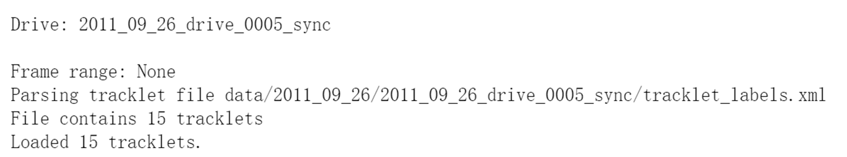
  date = '2011_09_26'
  drive = '0005'
  dataset = load_dataset(date, drive)
  tracklet_rects, tracklet_types = load_tracklets_for_frames(len(list(dataset.velo)), '/home/ecs-user/aliyun/Visualizing-lidar-data/data/{}/{}_drive_{}_sync/tracklet_labels.xml'.format(date, date, drive))

  输出结果如图所示，其中包含了15个对象的轨迹数据。

  

• 6、绘制图像

  定义draw_box函数，在坐标系中绘制3D点云并为物体绘制3D边框。分别绘制相机数据、3D点云和平面点云。

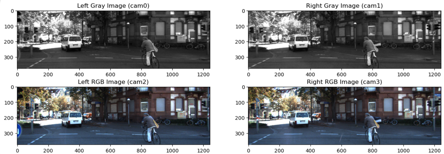
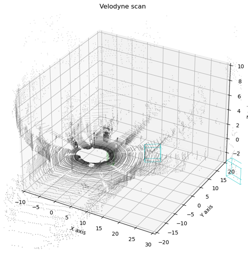
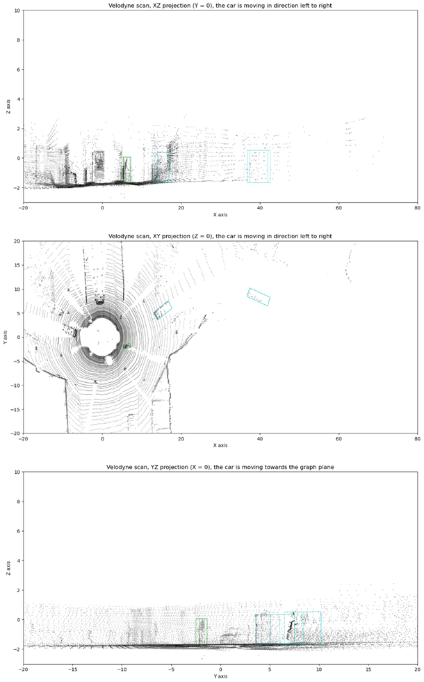
  import matplotlib.pyplot as plt
  from mpl_toolkits.mplot3d import Axes3D
  
  colors = {
      'Car': 'b',
      'Tram': 'r',
      'Cyclist': 'g',
      'Van': 'c',
      'Truck': 'm',
      'Pedestrian': 'y',
      'Sitter': 'k'
  }
  axes_limits = [
      [-20, 80], # X axis range
      [-20, 20], # Y axis range
      [-3, 10]   # Z axis range
  ]
  axes_str = ['X', 'Y', 'Z']
  
  def draw_box(pyplot_axis, vertices, axes=[0, 1, 2], color='black'):
      vertices = vertices[axes, :]
      connections = [
          [0, 1], [1, 2], [2, 3], [3, 0],  # Lower plane parallel to Z=0 plane
          [4, 5], [5, 6], [6, 7], [7, 4],  # Upper plane parallel to Z=0 plane
          [0, 4], [1, 5], [2, 6], [3, 7]  # Connections between upper and lower planes
      ]
      for connection in connections:
          pyplot_axis.plot(*vertices[:, connection], c=color, lw=0.5)
  
  def display_frame_statistics(dataset, tracklet_rects, tracklet_types, frame, points=0.2):
      dataset_gray = list(dataset.gray)
      dataset_rgb = list(dataset.rgb)
      dataset_velo = list(dataset.velo)
      
      print('Frame timestamp: ' + str(dataset.timestamps[frame]))
      # 绘制相机数据
      f, ax = plt.subplots(2, 2, figsize=(15, 5))
      ax[0, 0].imshow(dataset_gray[frame][0], cmap='gray')
      ax[0, 0].set_title('Left Gray Image (cam0)')
      ax[0, 1].imshow(dataset_gray[frame][1], cmap='gray')
      ax[0, 1].set_title('Right Gray Image (cam1)')
      ax[1, 0].imshow(dataset_rgb[frame][0])
      ax[1, 0].set_title('Left RGB Image (cam2)')
      ax[1, 1].imshow(dataset_rgb[frame][1])
      ax[1, 1].set_title('Right RGB Image (cam3)')
      plt.show()
  
      points_step = int(1. / points)
      point_size = 0.01 * (1. / points)
      velo_range = range(0, dataset_velo[frame].shape[0], points_step)
      velo_frame = dataset_velo[frame][velo_range, :]      
      def draw_point_cloud(ax, title, axes=[0, 1, 2], xlim3d=None, ylim3d=None, zlim3d=None):
          ax.scatter(*np.transpose(velo_frame[:, axes]), s=point_size, c=velo_frame[:, 3], cmap='gray')
          ax.set_title(title)
          ax.set_xlabel('{} axis'.format(axes_str[axes[0]]))
          ax.set_ylabel('{} axis'.format(axes_str[axes[1]]))
          if len(axes) > 2:
              ax.set_xlim3d(*axes_limits[axes[0]])
              ax.set_ylim3d(*axes_limits[axes[1]])
              ax.set_zlim3d(*axes_limits[axes[2]])
              ax.set_zlabel('{} axis'.format(axes_str[axes[2]]))
          else:
              ax.set_xlim(*axes_limits[axes[0]])
              ax.set_ylim(*axes_limits[axes[1]])
          if xlim3d!=None:
              ax.set_xlim3d(xlim3d)
          if ylim3d!=None:
              ax.set_ylim3d(ylim3d)
          if zlim3d!=None:
              ax.set_zlim3d(zlim3d)
              
          for t_rects, t_type in zip(tracklet_rects[frame], tracklet_types[frame]):
              draw_box(ax, t_rects, axes=axes, color=colors[t_type])
              
      # 绘制点云3D图像
      f2 = plt.figure(figsize=(15, 8))
      ax2 = f2.add_subplot(111, projection='3d')                    
      draw_point_cloud(ax2, 'Velodyne scan', xlim3d=(-10,30))
      plt.show()
      
      # 绘制点云平面图像
      f, ax3 = plt.subplots(3, 1, figsize=(15, 25))
      draw_point_cloud(
          ax3[0], 
          'Velodyne scan, XZ projection (Y = 0), the car is moving in direction left to right', 
          axes=[0, 2] # X and Z axes
      )
      draw_point_cloud(
          ax3[1], 
          'Velodyne scan, XY projection (Z = 0), the car is moving in direction left to right', 
          axes=[0, 1] # X and Y axes
      )
      draw_point_cloud(
          ax3[2], 
          'Velodyne scan, YZ projection (X = 0), the car is moving towards the graph plane', 
          axes=[1, 2] # Y and Z axes
      )
      plt.show()
    
  frame = 10
  
  display_frame_statistics(dataset, tracklet_rects, tracklet_types, frame)

  分别读取并显示数据集中cam0和cam1的RGB图以及灰度图。

  

  绘制3D点云。

  

  

• 7、绘制三维图

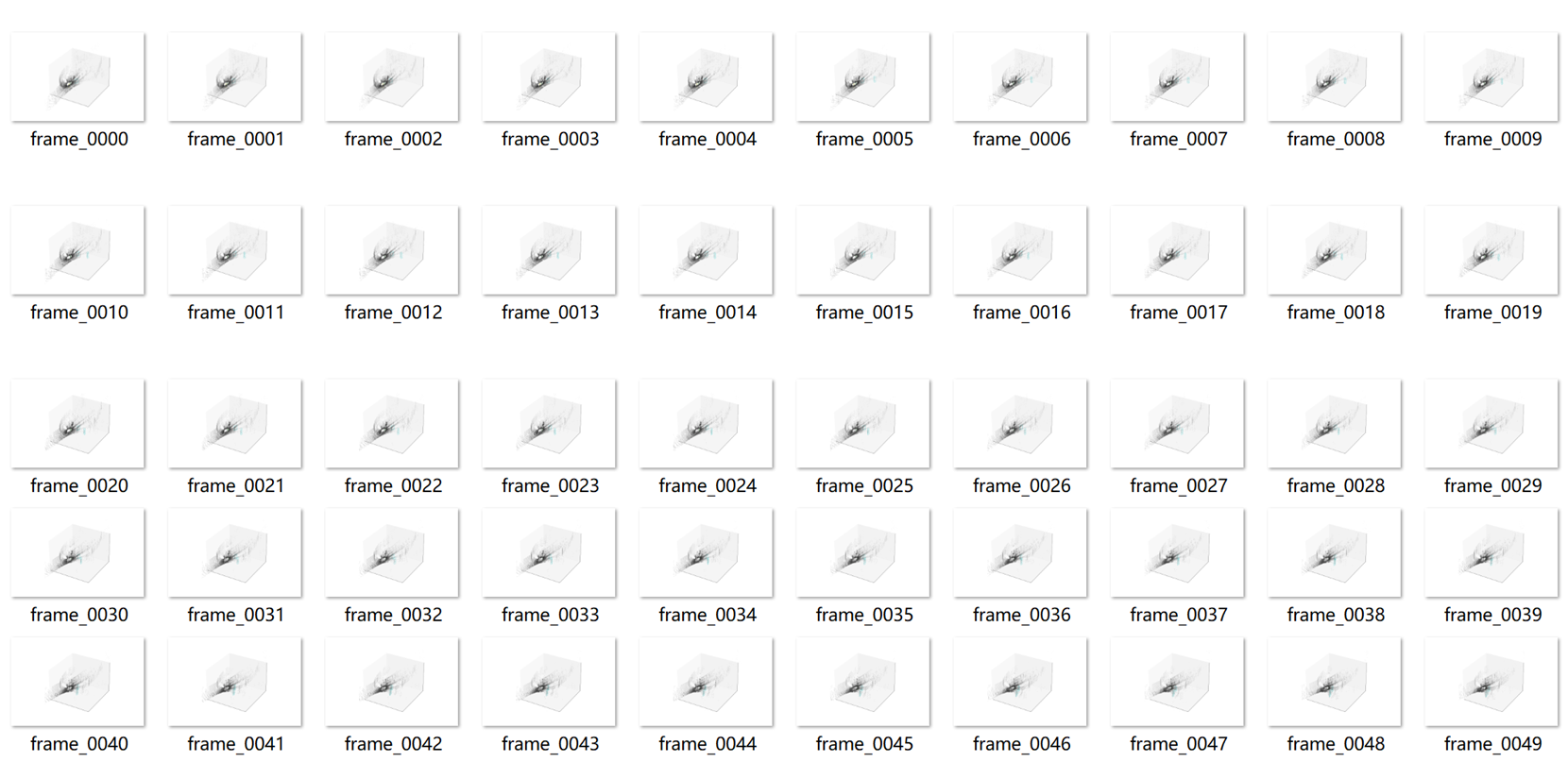
  将每一帧的雷达数据绘制成一幅三维图，并保存在pictures文件夹中。

  from utilities import print_progress
  from moviepy import ImageSequenceClip
  
  def draw_3d_plot(frame, dataset, tracklet_rects, tracklet_types, points=0.2):
      dataset_velo = list(dataset.velo)
      
      f = plt.figure(figsize=(12, 8))
      axis = f.add_subplot(111, projection='3d', xticks=[], yticks=[], zticks=[])
  
      points_step = int(1. / points)
      point_size = 0.01 * (1. / points)
      velo_range = range(0, dataset_velo[frame].shape[0], points_step)
      velo_frame = dataset_velo[frame][velo_range, :]
      axis.scatter(*np.transpose(velo_frame[:, [0, 1, 2]]), s=point_size, c=velo_frame[:, 3], cmap='gray')
      axis.set_xlim3d(*axes_limits[0])
      axis.set_ylim3d(*axes_limits[1])
      axis.set_zlim3d(*axes_limits[2])
      for t_rects, t_type in zip(tracklet_rects[frame], tracklet_types[frame]):
          draw_box(axis, t_rects, axes=[0, 1, 2], color=colors[t_type])
      filename = '/home/ecs-user/aliyun/Visualizing-lidar-data/pictures/frame_{0:0>4}.png'.format(frame)
      plt.savefig(filename)
      plt.close(f)
      return filename

  生成的三维图文件如图所示。

  

• 8、制作GIF文件

  将保存在pictures文件夹中的三维图保存为一个GIF文件。

  frames = []
  n_frames = len(list(dataset.velo))
  
  print('Preparing animation frames...')
  for i in range(n_frames):
      print_progress(i, n_frames - 1)
      filename = draw_3d_plot(i, dataset, tracklet_rects, tracklet_types)
      frames += [filename]
  print('...Animation frames ready.')
  
  clip = ImageSequenceClip(frames, fps=5)
  % time
  clip.write_gif('/home/ecs-user/aliyun/Visualizing-lidar-data/pcl_data.gif', fps=5)

  合成的GIF文件保存在对应路径中。

  

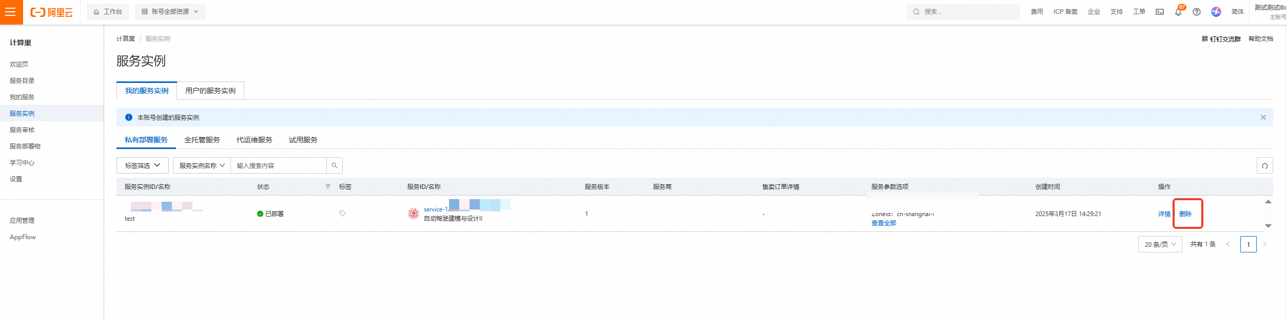
清理资源

• 计算巢—服务实例—复制服务实例ID，点击【删除】

  

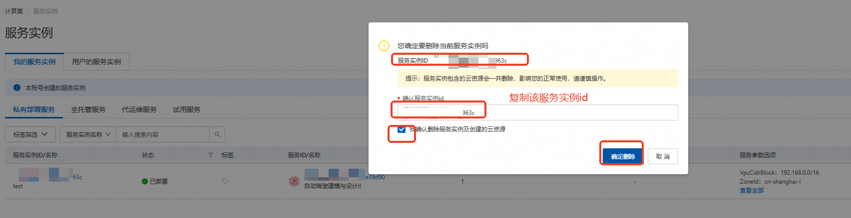
• 在弹窗粘贴服务实例ID，并进行勾选，点击【确定删除】

  

• 完成安全验证后，即可成功释放实例。

  

• 回到云服务器ECS——实例，检查是否成功释放资源

  

关闭实验

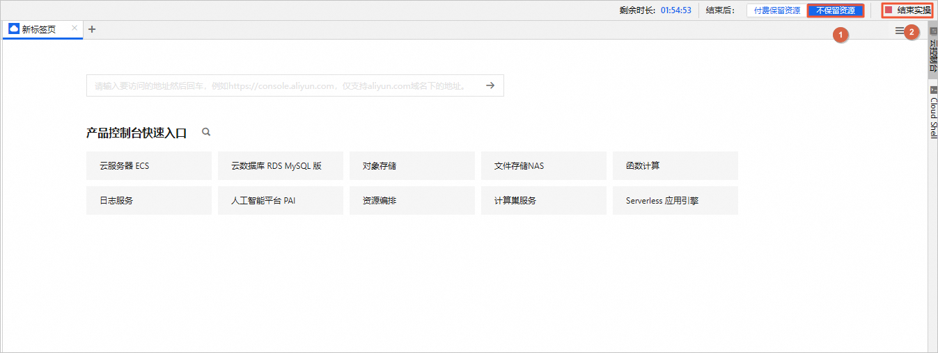
• 在完成实验后，如果无需继续使用资源，选择不保留资源，单击结束实操。在结束实操对话框中，单击确定。

  

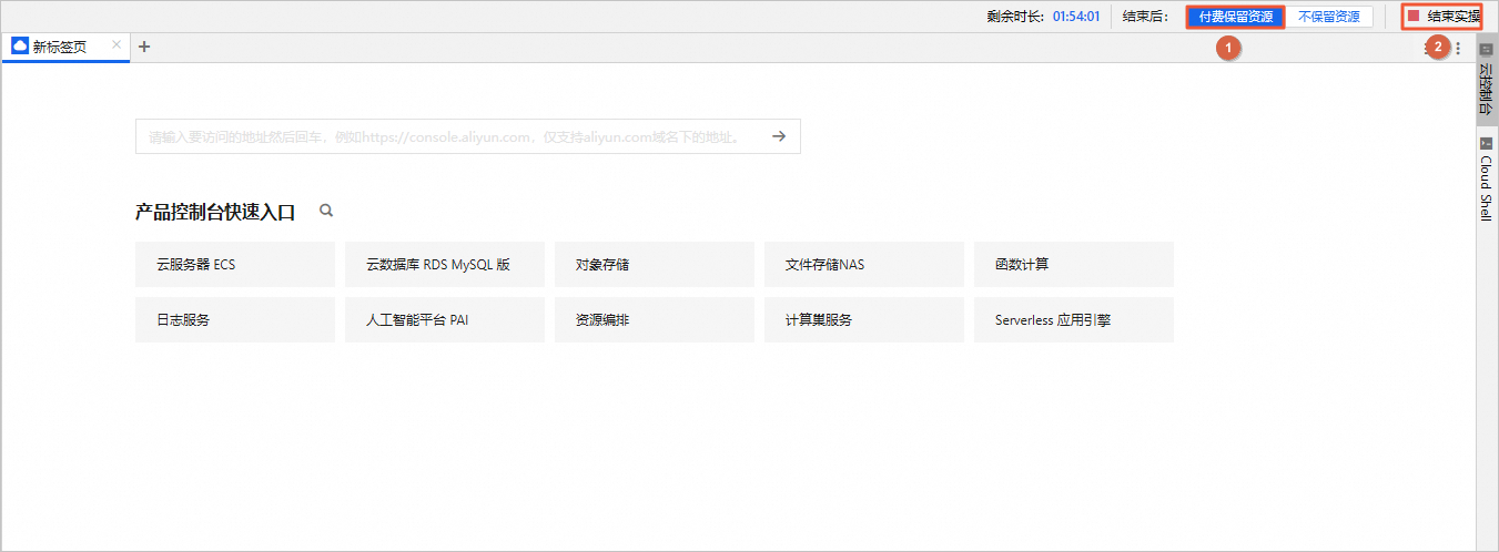
• 在完成实验后，如果需要继续使用资源，选择付费保留资源，单击结束实操。在结束实操对话框中，单击确定。请随时关注账户扣费情况，避免发生欠费。