Continuous performance profiling helps you identify performance bottlenecks in your Python applications, such as high CPU usage and memory consumption. It provides detailed statistics by method name, class name, and line number to help you optimize your code, reduce latency, increase throughput, and lower costs. This topic describes how to enable continuous performance profiling for Python applications in ARMS and how to view the profiling data.
Prerequisites
The continuous performance profiling feature is available only in Expert Edition and the pay-by-written-data-volume billing mode. To subscribe to Expert Edition, see pay-as-you-go. To switch to the pay-by-written-data-volume billing mode, see Change billing method.
To request access to this feature in these regions, join our DingTalk group (ID: 22560019672).
Continuous performance profiling data is retained for only 7 days.
You must first integrate your application and update the Python Agent to version 2.3.0 or later. You can check the agent version on the Application Settings > Agent Management page and refer to Specify a version.
If your Virtual Private Cloud (VPC) network has a bucket policy that restricts access to Object Storage Service (OSS), you must update your policy. This feature uploads collected application data to a centralized ARMS OSS bucket for storage and analysis. If your policy does not include this bucket, data collection will fail. To ensure data is collected, add the continuous performance profiling bucket,
arms-profiling-<regionId>, to your policy rules. Replace<regionId>with your application's region ID. For example, if your application is deployed in the China (Hangzhou) region, the bucket isarms-profiling-cn-hangzhou.
Supported Python versions
Enable continuous performance profiling
Log on to the ARMS console. In the left-side navigation pane, choose Application Monitoring > Application List.
On the Application List page, select a region in the top navigation bar and click the name of your application.
At the top of the Application List page, select the target region, and then click the target application name.
NoteThe icons in the Language column represent the following:
 : A Java application connected to Application Monitoring.
 : A Go application connected to Application Monitoring.
 : A Python application connected to Application Monitoring.
-: An application connected to Managed Service for OpenTelemetry.
In the top navigation bar, choose Application Settings > Custom Settings.
In the Continuous Profiling section, enable the master switch and other features as needed.
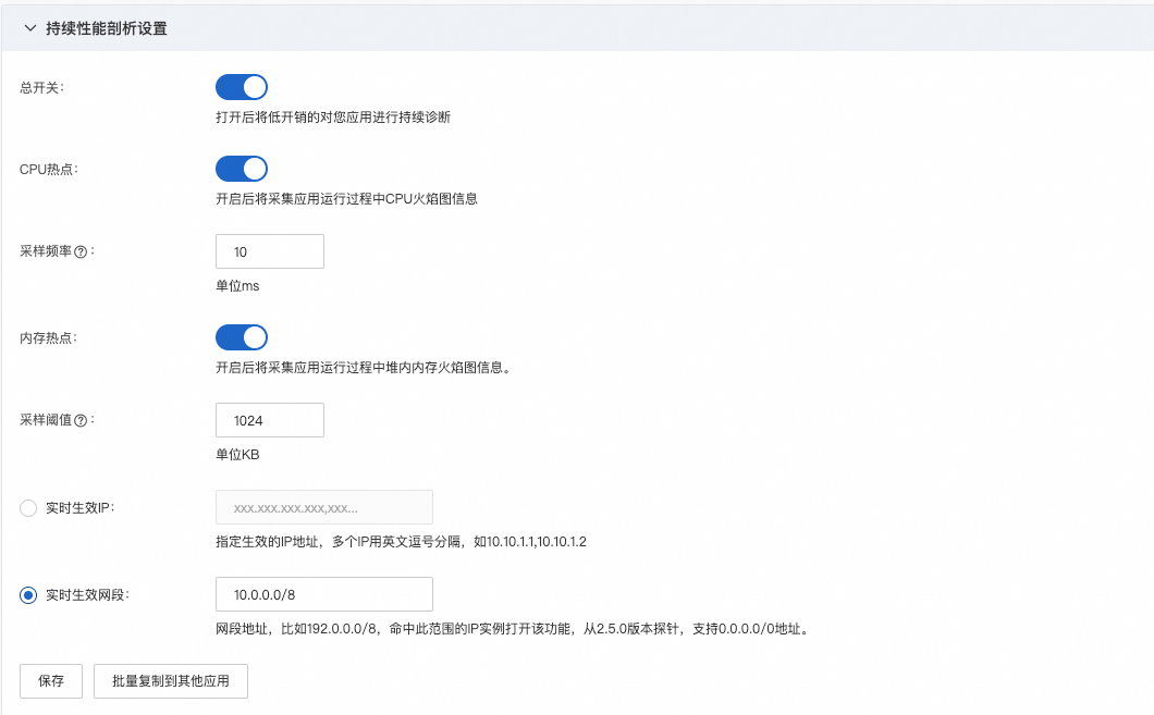
The Continuous Profiling section contains the following settings: Master Switch (enables low-overhead continuous diagnosis), CPU Hotspots (collects CPU flame graph data), Sampling Frequency (in ms, default is 10), Memory Hotspots (collects heap memory flame graph data), Sampling Threshold (in KB, default is 1024), and more.
The settings take about 2 minutes to take effect.
View continuous performance profiling data
View Continuous Performance Profiling Data
Log on to the ARMS console. In the left-side navigation pane, choose .
Go to the ARMS console > , click your application, and choose in the top navigation bar.
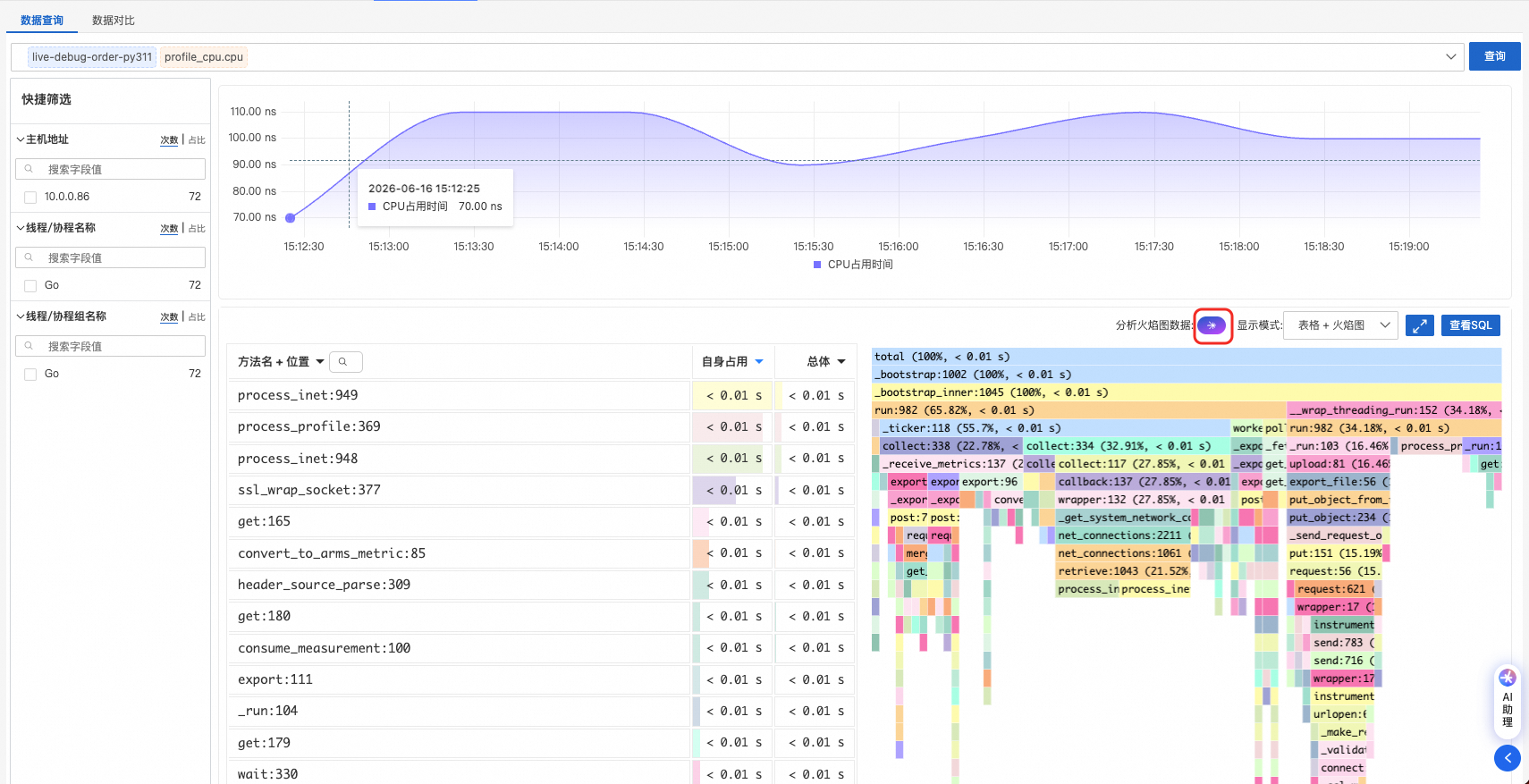
Data query
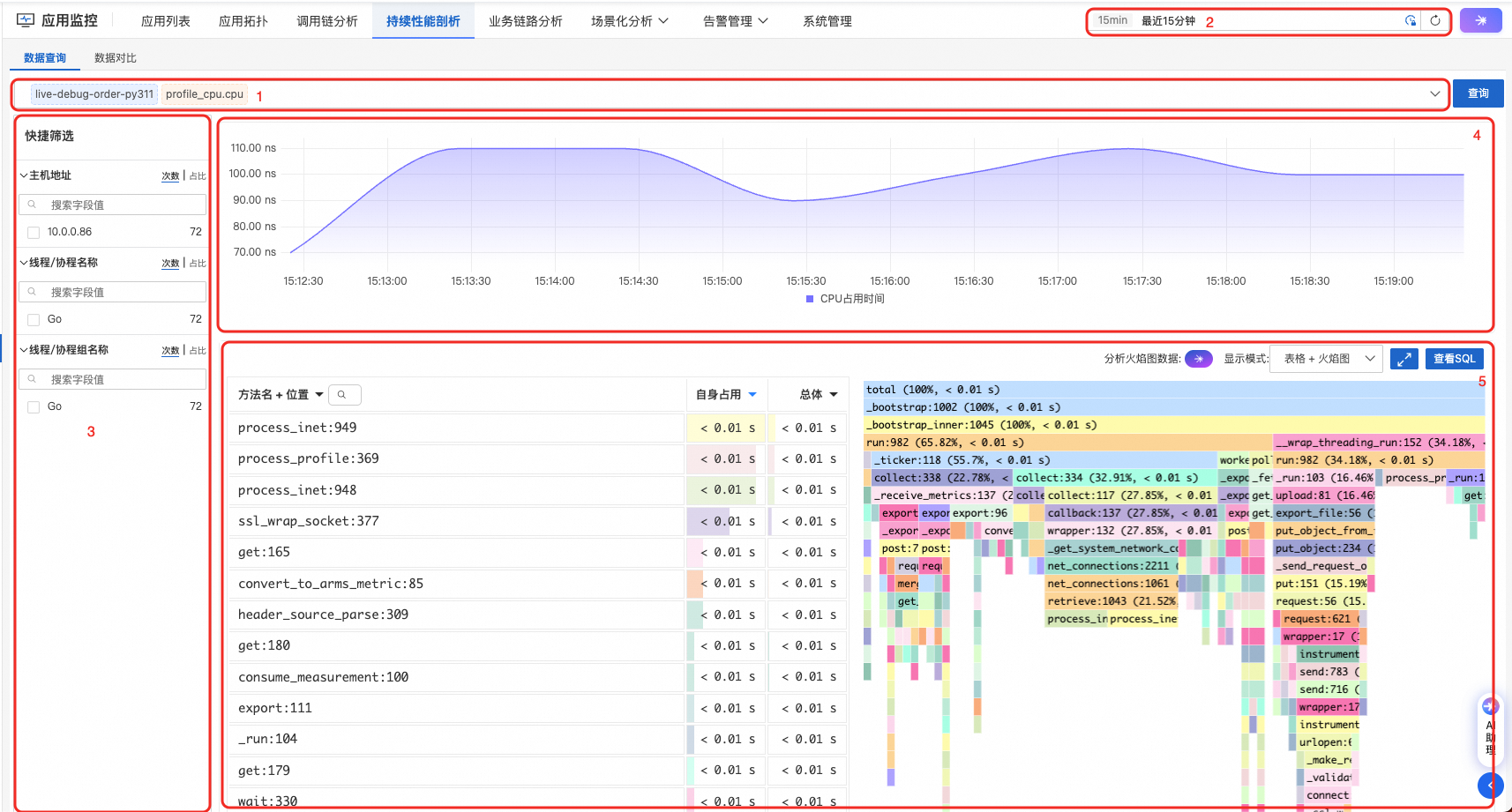
Filter metadata (① in the figure)
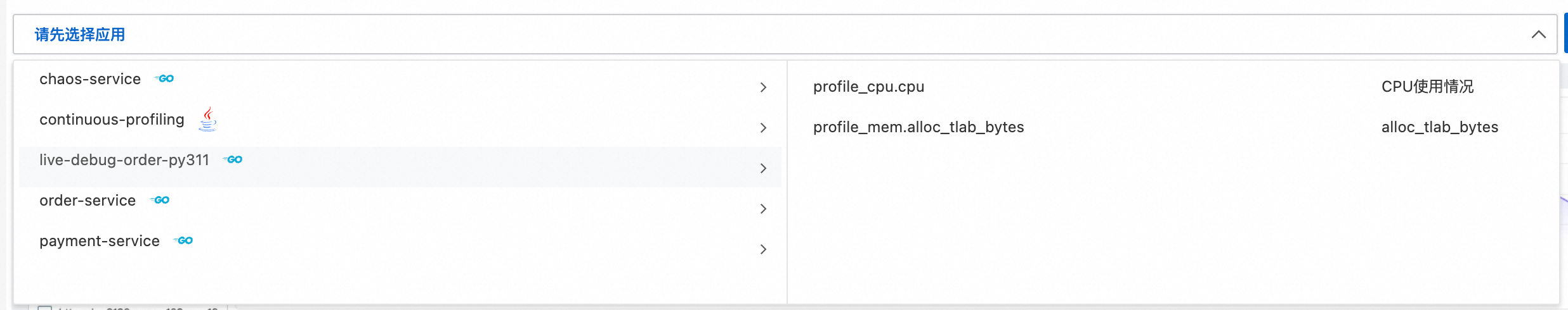
Profile metadata consists of an application name and a profile type. These two parts identify a set of profiles.
After you select a metadata set, the system automatically updates the trend chart and flame graph.
NoteIf you change the selected metadata, any existing tag filters in the Quick Filter area are cleared.
The metadata selection area is divided into two columns. The left column lists connected applications, and the right column displays the available profile types and their descriptions.
Set the time range for the metadata (② in the figure)
This time range specifies the period for which to retrieve metadata and quick filter data. To ensure a fast response, the default is the last 15 minutes. You typically do not need to change this setting. However, you can adjust it if the data changes frequently or has large gaps.
This setting filters the data shown in the trend chart and flame graph by time but does not change the selected application or profile type. It supports auto-refresh.
Quick Filter (③ in the figure)
The data for quick labels depends on the time range of the metadata. Label keys are sourced from the
labelsfield (in JSON format) of the performance monitoring data. A logical AND relationship is applied across different labels. Once you select labels, the system automatically updates the trend chart and flame graph accordingly.host IP: The IP address of the profiled instance.
thread name: All threads of the application. You can use this to find abnormal threads based on CPU time, memory usage, and other metrics.
thread group name: A collection of threads that follow the same rules. You can use this to find a class of abnormal threads based on CPU time, memory usage, and other metrics.
Trend chart (④ in the figure)
Shows the trend of the selected profile metadata over the specified time range.
Flame graph (⑤ in the figure)
After you select the metadata, tags, and time range, the system automatically generates a flame graph for the profile set.
Click the
 icon to view Copilot's analysis and suggestions for the current flame graph. You can also ask custom questions about CPU, memory, and flame graph data.
Select a Display mode: Flame Graph Only, Table Only, or Table+Flame Graph.
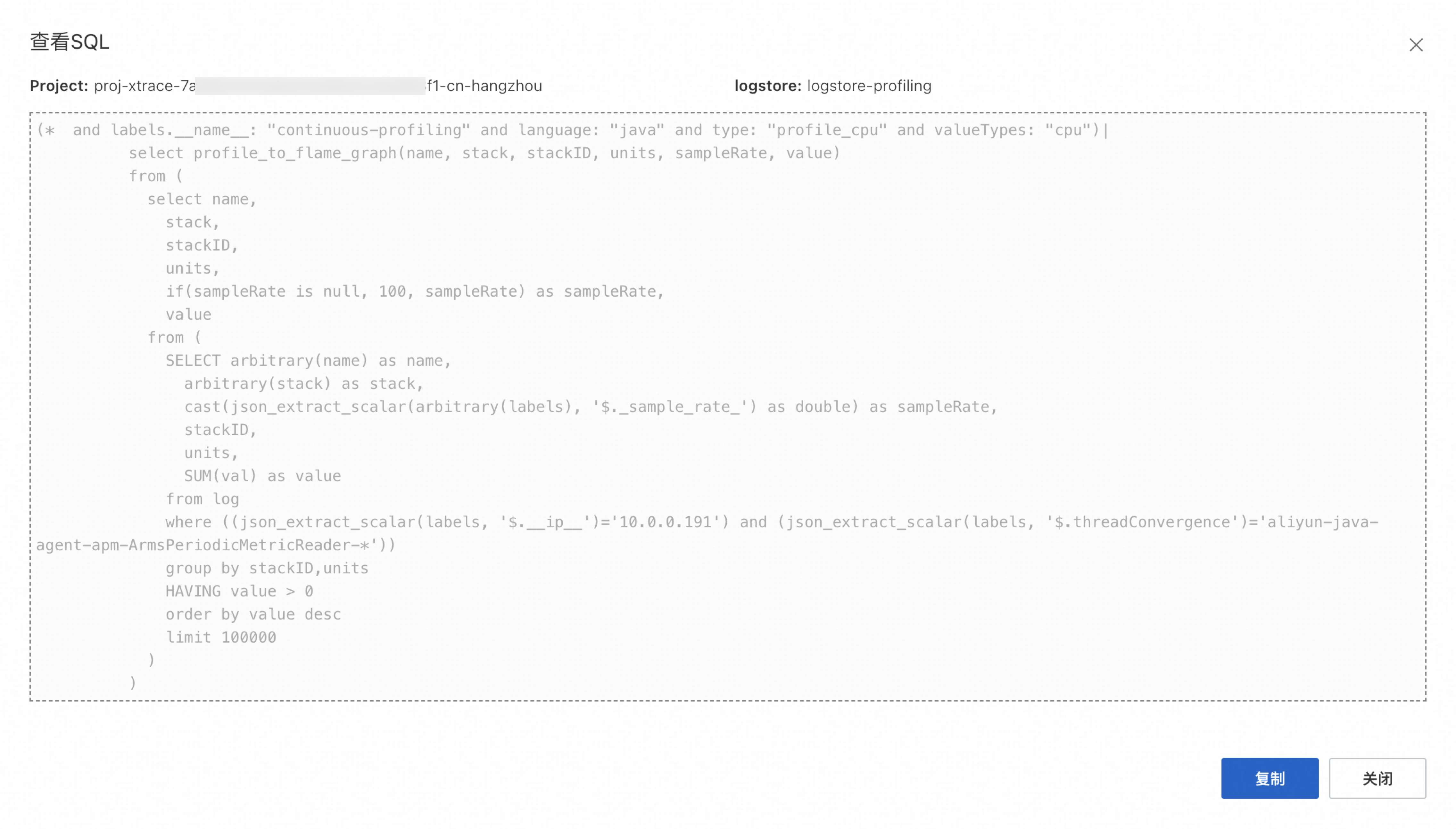
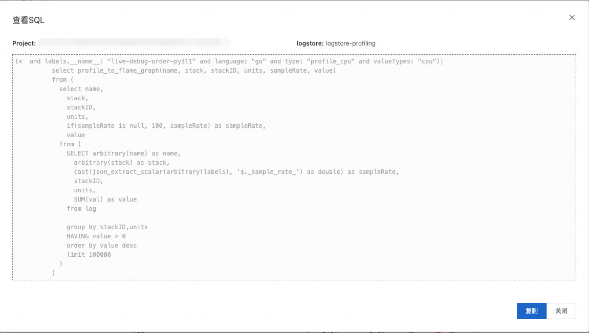
Click View SQL to see the SQL query used to build the flame graph. You can use this query to analyze the data in the corresponding Project and Logstore of Log Service (SLS).
Data comparison
Data comparison lets you compare a profile's performance data between two time periods.
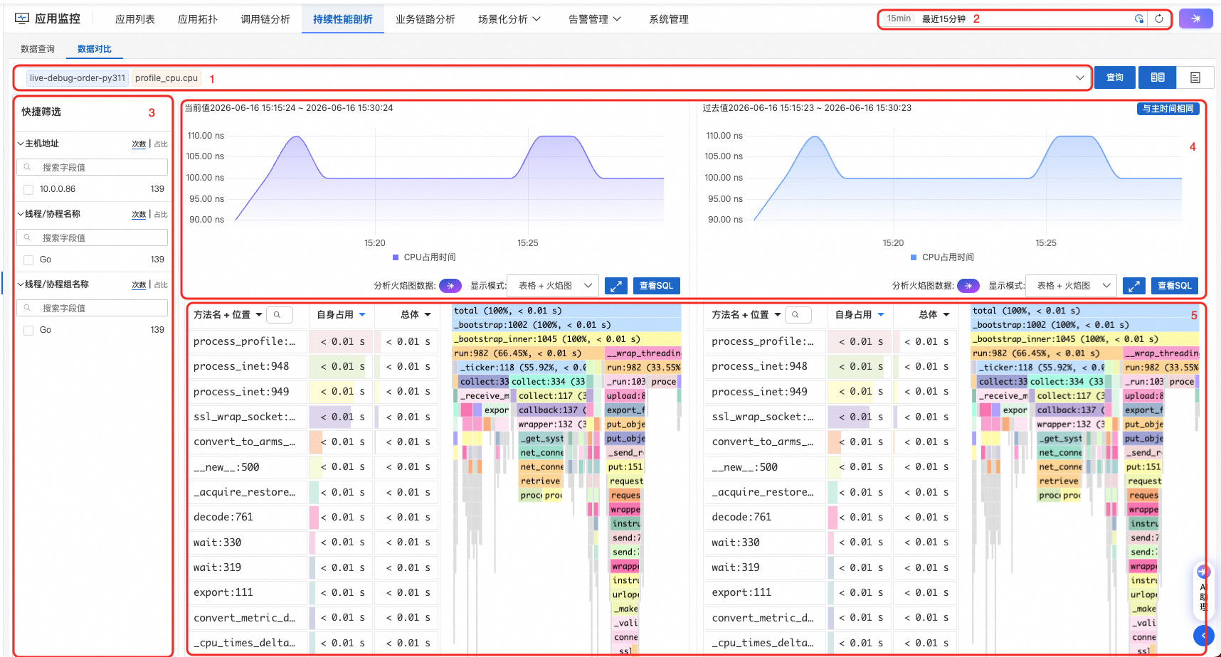
Filter metadata (① in the figure)
Profile metadata consists of an application name and a profile type. These two parts identify a set of profiles.
After you select a metadata set, the system automatically updates the trend chart and flame graph.
NoteIf you change the selected metadata, any existing tag filters in the Quick Filter area are cleared.
The metadata selection area is divided into two columns. The left column lists connected applications, and the right column displays the available profile types and their descriptions. After making your selections, click Query to compare the data.
Set the time range for the metadata (② in the figure)
This time range specifies the period for which to retrieve metadata and quick filter data. To ensure a fast response, the default is the last 15 minutes. You typically do not need to change this setting. However, you can adjust it if the data changes frequently or has large gaps.
This setting affects only the time range of the trend chart and flame graph, not the metadata itself. It supports auto-refresh.
Quick Filter (③ in the figure)
The data for quick tags depends on the time range of the metadata. The tag keys are sourced from the
labelsfield (in JSON format) in the performance monitoring data. A logical AND relationship exists between different tags. After you select tags, the system automatically updates the trend chart and flame graph based on your selection.host IP: The IP address of the profiled instance.
thread name: All threads of the application. You can use this to find abnormal threads based on CPU time, memory usage, and other metrics.
thread group name: A collection of threads that follow the same rules. You can use this to find a class of abnormal threads based on CPU time, memory usage, and other metrics.
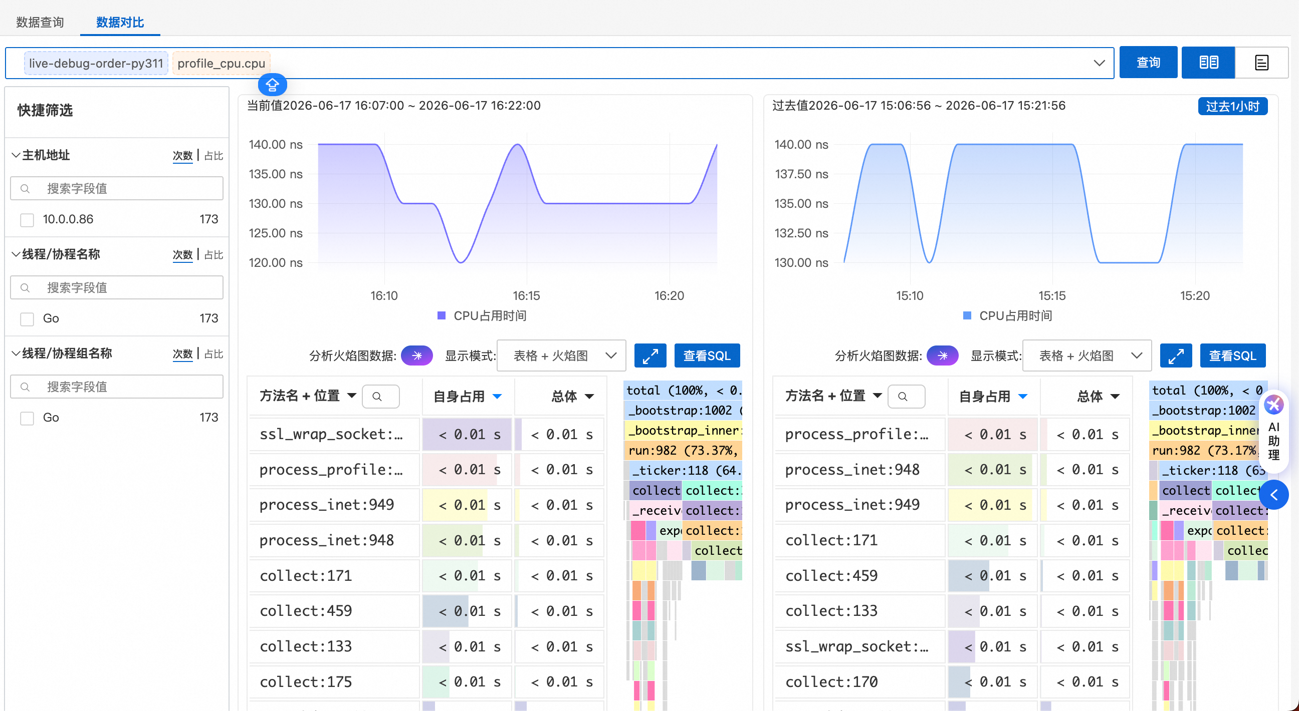
Trend chart (④ in the figure)
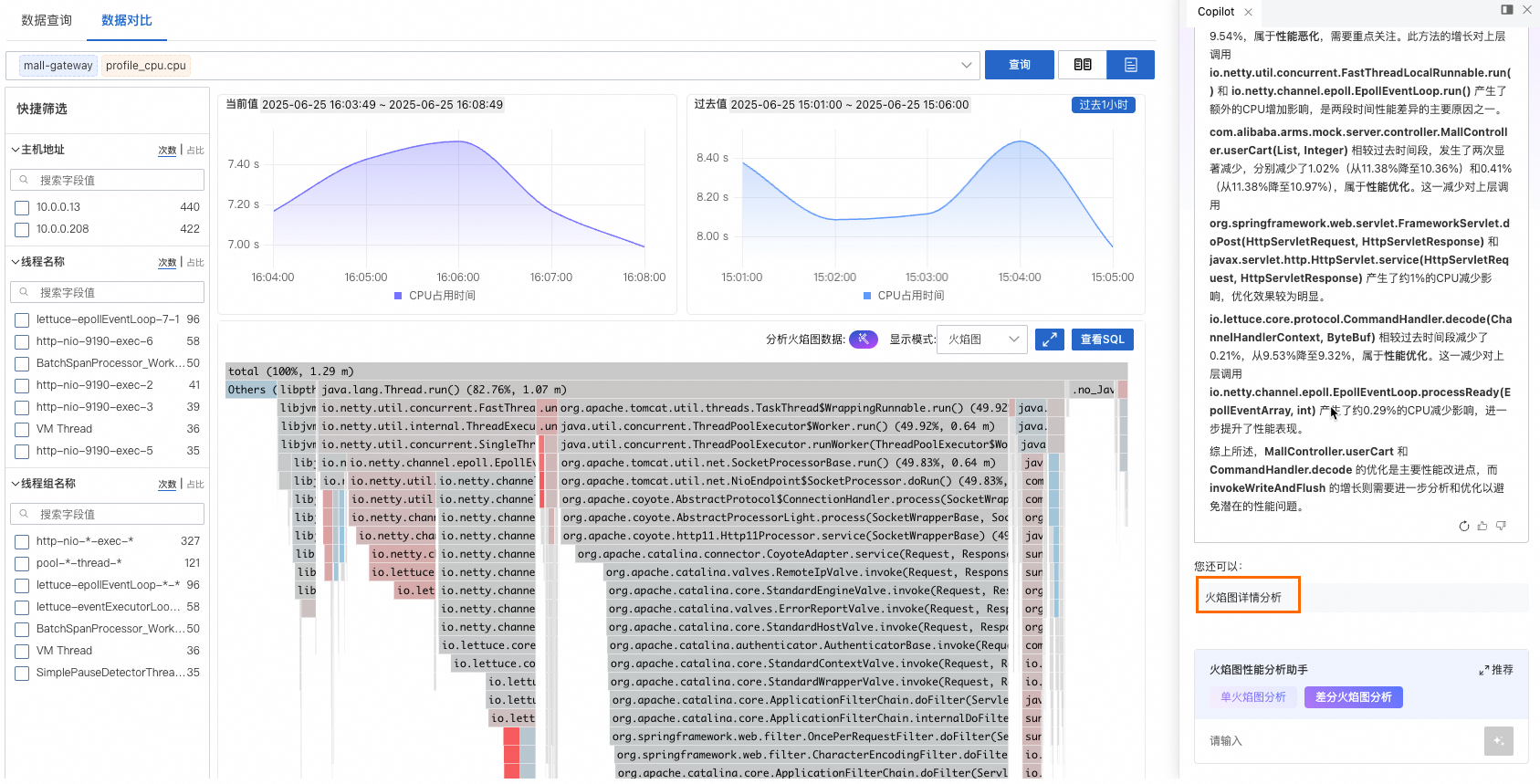
The trend chart displays the overall performance trends for the current and past time periods. The chart is based on the filtered metadata and tags, aggregated over time according to the policy specified in the metadata section.
In the Current Value area, the time range is fixed to the main time range (② in the figure). In the Past Value area, you can click Past N Hours to specify the comparison period.
Flame graph (⑤ in the figure)
A flame graph is automatically generated based on your selections. Click the
icon to switch between the Simple Comparison view and the Blended Comparison view.Simple comparison
The Simple Comparison view divides the page into two columns. The left column shows the trend chart and flame graph for the Current Value period, and the right column shows the data for the Past Value period. This allows for a direct comparison of performance data for each method between the two time periods.
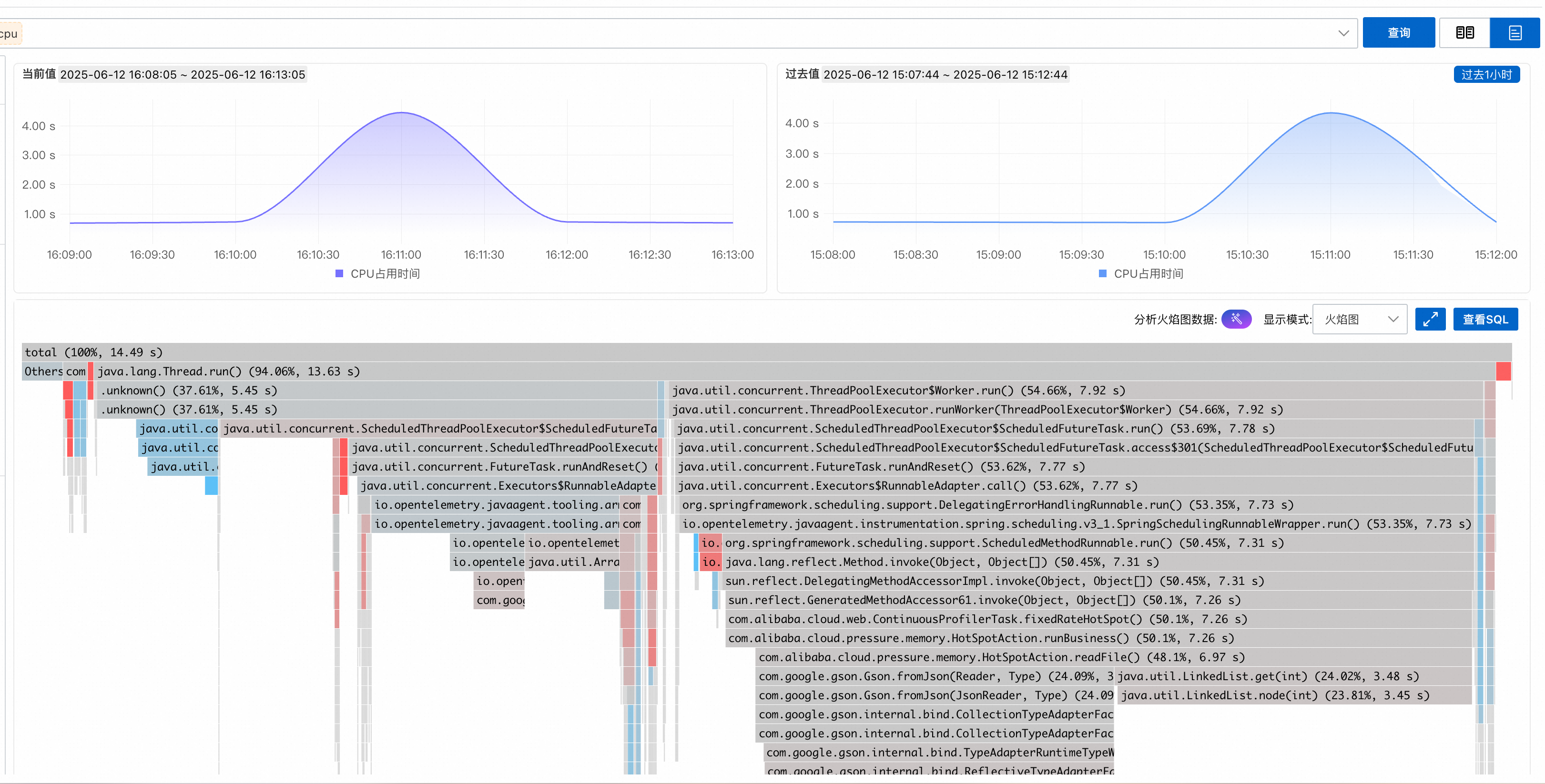
Blended comparison
Red indicates a relative increase in resource consumption compared to the past, while blue indicates a decrease.
This view merges the flame graphs from the two periods into a single chart.
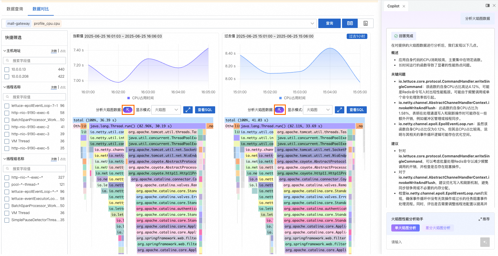
Click the
icon to view Copilot's analysis and suggestions for the current flame graph. You can also ask custom questions about CPU, memory, and flame graph data.In the Blended Comparison view, Copilot analyzes and compares the profiling data from the two time periods, highlighting performance changes and influencing factors in the comparison flame graph. Click Flame Graph Detail Analysis to have Copilot further analyze specific performance issues and provide recommendations.
Select a Display mode: Flame Graph Only, Table Only, or Table+Flame Graph.
Click View SQL to see the SQL query used to build the flame graph. You can use this query to analyze the data in the corresponding Project and Logstore of Log Service (SLS).