Prometheus is a popular open source project in the field of time series data monitoring and one of the most widely adopted projects under the Cloud Native Computing Foundation (CNCF). It efficiently collects and stores metrics and provides Prometheus Query Language (PromQL), a flexible query language for computing and analyzing time series data. However, developers are often confused by PromQL’s calculation results because its syntax differs significantly from traditional SQL. This topic uses illustrations to explain how PromQL calculations work and breaks down the calculation steps using specific query statements. Please point out any errors in this explanation of PromQL.
PromQL vs. SQL
Before we begin, we must agree on one point: PromQL is not SQL. It is a query language based on a non-precise model. Its syntax includes features such as backtracking for data points, boundary extrapolation, and window calculations. The following table summarizes the main differences between PromQL and SQL.
Comparison |
PromQL |
SQL |
Data model |
Based on time series: metric name + labels + timestamp + value. |
Based on tables: row + column. |
Index structure |
Relies on efficient indexing of labels. No manual management is required. |
Relies on database indexes. You must manually optimize the index policy. |
Basic syntax |
No SELECT statement. Directly operates on metrics, such as http_requests_total{job="api"}. |
Core structure is SELECT ... FROM ... WHERE .... |
Time/Filter conditions |
Reads all data points that match the time range and filter conditions. |
Reads all data points that match the time range and filter conditions. |
Pre-selected points |
Before calculation, pre-selects data points based on parameters such as lookback and window. |
None. |
Aggregation/Grouping |
Supports multiple aggregation operators with by or without for grouping, such as sum by (job). |
Uses aggregate functions, such as SUM() and AVG(), with GROUP BY for grouping. |
JOIN/Association |
Uses operators such as on/ignoring and group_left/group_right to match labels. This is similar to a many-to-one association. |
Uses JOIN operators, such as INNER JOIN and LEFT JOIN, to explicitly associate data from two tables. |
Subquery |
Supports subqueries, such as avg_over_time(rate(http_requests[5m])[1h:1m]) |
Supports subqueries, such as SELECT * FROM (SELECT ... FROM ... WHERE ...) WHERE ... |
Result type |
Returns a vector or matrix. |
Returns tabular data (rows and columns). |
How PromQL works: A visual guide
All calculations in PromQL revolve around the concept of a "timeline." First, let's understand what a timeline is. In a time series scenario, the monitored object is a "metric." For example, the metric process_resident_memory_bytes represents the resident memory usage of a process. In the Prometheus data model, a set of Key-Value pairs represents an independent timeline. This timeline consists of a metric and a list of labels:
Metric: The
Keyfor the metric is fixed as"__name__". TheValueis the corresponding "MetricName", which is the metric name.Labels: The label list is a set of key-value pairs that act as secondary dimension properties. For example,
job="demo", instance="demo.promlabs.com:10000"represents a process named "demo" on a machine instance with the address "demo.promlabs.com:10000".
Besides the metric and labels, a single monitoring data point also consists of a timestamp and a value. These represent the collection time and the value of the monitoring point. The following figure shows an example. Its PromQL statement is process_resident_memory_bytes{}/1024/1024. The figure shows three timelines:
__name__="process_resident_memory_bytes", instance="demo.promlabs.com:10000", job="demo"__name__="process_resident_memory_bytes", instance="demo.promlabs.com:10001", job="demo"__name__="process_resident_memory_bytes", instance="demo.promlabs.com:10002", job="demo"
The monitoring value in each timeline changes over time. This clearly shows how a monitored object changes over time.
The previous example only performed a simple query on the metric process_resident_memory_bytes. It did not involve PromQL's various aggregation operators (such as avg/sum/count/max/min), window functions (such as rate/increase/avg_over_time/sum_over_time), non-window functions (such as abs/clamp/round/sort/label_replace), vector matching (such as group_left/group_right), binary expressions, or subqueries. For a complete list of supported syntax features, see Querying Prometheus.
The PromQL query API supported by Prometheus mainly includes the following four input parameters:
start/end: The query time range.
query: The PromQL query statement.
step: The step size. This parameter indicates the execution interval for each calculation round.
The unique concept of step
We mentioned earlier that "PromQL is a non-precise query language." This is largely related to the step parameter in the PromQL compute engine. The step parameter indicates the execution interval for each calculation round within the specified time range [start, end]. The figure below shows how the step parameter works. The start parameter is "10:00:00", the end parameter is "10:11:30", and the step parameter is "120s". The calculation process can be summarized as follows: from the start time to the end time, a calculation round is executed at each step interval. In this example, the first calculation is at "10:00:00", and the sixth is at "10:10:00". The expected seventh round would be after the given end time, so only six rounds of calculation are performed.
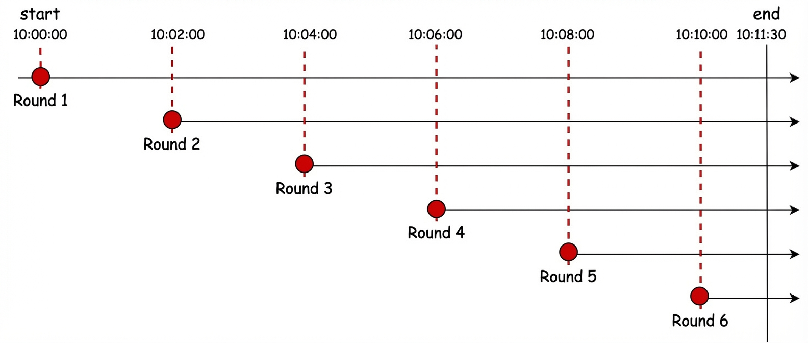
We must emphasize one point here. In the Prometheus compute engine, all types of PromQL statement calculations, including all aggregation operators, functions, and binary operations, follow this main premise: "perform multiple rounds of calculation at step intervals." From a calculation process perspective, the step parameter can often be seen as a special design to "reduce query precision." This is especially true for queries over long periods, where the step parameter can be as high as several hours, such as 1h or 1d. In such scenarios, the calculation process often skips data from many time intervals. This causes the calculation results to show only the general trend of the metric.
Special data point selection
In regular SQL calculations, all data points that fall within the input time period [start, end] and meet the WHERE conditions are included in the calculation process. PromQL's calculation is very different. In each calculation round at the "step" interval, the data points included in the actual calculation must go through a special "selection" logic. There are two main ways to "select" points: lookback selection based on the lookback-delta parameter, and range selection based on the window function's input parameter [xx].
Lookback selection
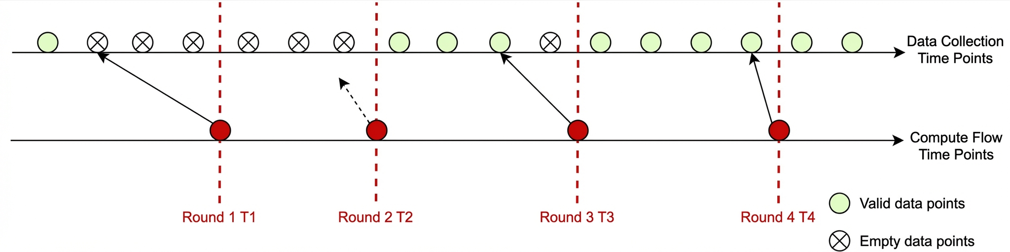
The data collection side of a time series usually collects and reports monitoring data at fixed intervals. However, the input parameters for PromQL queries are often executed arbitrarily. In most cases, they do not coincide exactly with the reporting timestamps. The PromQL calculation process starts from the input startTime and ends at the endTime. If there is no raw data point at the time T of each round, it will look back to find the most recent data point to use as the data for time T. At time T2, no valid data point was selected.
The figure below shows a complete example of the "selection" process for a single timeline. Using the parameters start "10:00:00", end "10:11:30", step "120s" as an example, assume the raw monitoring data is reported every "30s". The entire process involves six rounds of selection. The final selected timestamps are: "09:59:40", "10:01:40", "10:03:40", "10:05:40", "10:07:40", and "10:09:40". The PromQL-Engine treats the data points at these six timestamps as the data points for "10:00:00", "10:02:00", "10:04:00", "10:06:00", "10:08:00", and "10:10:00", respectively. These points then enter the subsequent calculation process.
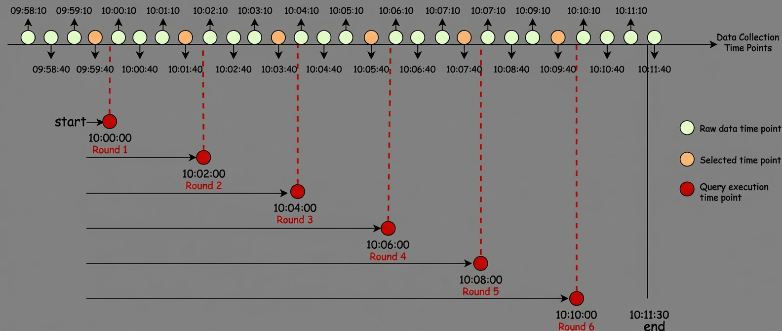
In the example above, the maximum time range for looking back to select a point is controlled by the lookback-delta parameter. This parameter defaults to 5 minutes in Prometheus and 3 minutes in SLS Metricstore. For example, at the "10:00:00" timestamp, the system looks back a maximum of 3 minutes. If no data point is found in the "09:57:00" to "10:00:00" interval, it means there is no data for the "10:00:00" timestamp to enter the next stage of calculation. This selection mode corresponds to the InstantVectorSelector in Prometheus, which is defined as VectorSelector in the Prometheus source code.
Window function selection
As the name suggests, "window function selection" means this "selection" logic exists only in the calculation process of window functions. Using the same parameters as before, start "10:00:00", end "10:11:30", step "120s", let's also assume the window function's window parameter is [5m]. This parameter represents 5 minutes.
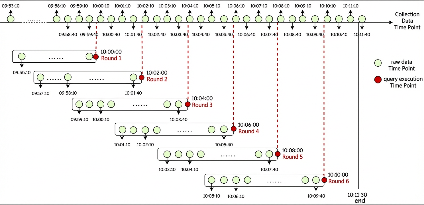
As shown in the figure above, each round of selection takes all data points from the preceding 5-minute window. For example, in the first round of selection, the execution time is "10:00:00". In this round, the 10 data points within the "09:55:00" to "10:00:00" window ("09:55:10", "09:55:40", "09:56:10", "09:56:40", "09:57:10", "09:57:40", "09:58:10", "09:58:40", "09:59:10", "09:59:40") are all included in the subsequent calculation. This selection mode corresponds to the RangeVectorSelector in Prometheus, which is defined as MatrixSelector in the Prometheus source code.
Compute engine
Before we discuss the various specific PromQL calculation operations, let's re-emphasize the main premise mentioned earlier: All types of PromQL statement calculations, including all aggregation operators, functions, and binary operations, follow this main premise: "perform multiple rounds of calculation at step intervals." This section will use illustrations to introduce several common calculation operations in PromQL syntax.
Filter queries
This type of basic query statement does not involve any operators, functions, or expressions. The query statement supports adding filter conditions to any label. It only supports the =, !=, =~, and !~ matching operators. Filter conditions are usually pushed down to the storage tier. This means the data entering the calculation process has already been filtered.
The subsequent operations on the metric data are very simple. Simply select points using the lookback-delta mechanism. Here are a few query examples for reference.
http_requests_total{replica="rep-a"}
http_requests_total{replica!~".*a"}
http_requests_total{environment=~"staging|testing|development",method!="GET"}
If you do not want to specify a particular metric and want to include the metric name in the fuzzy matching condition, see the following example.
Note: Fuzzy matching on metric names is inefficient. We do not recommend it for production environments.
{__name__="http_requests_total", replica="rep-a"}
{__name__=~"http.*", replica="rep-a"}
{__name__=~".+", instance=~"127.*"}
Aggregation operators
Note: The calculation process for all aggregation operations can be summarized as "first select points using the lookback-delta mechanism, then perform aggregation across timelines."
The aggregation operators currently supported by PromQL are: sum, avg, min, max, bottomk, topk, group, count, count_values, stddev, stdvar, quantile, limitk, and limit_ratio. This section uses the max and count operators and the following three timelines to explain the calculation process of aggregation operators.
timeseries 1: __name__="request_total_count", instance="127.0.0.1:10000", job="prometheus"
timeseries 2: __name__="request_total_count", instance="127.0.0.1:10001", job="vm-agent"
timeseries 3: __name__="request_total_count", instance="127.0.0.1:10002", job="vm-agent"
The query input parameters are set as follows:
start: 10:00:00
end : 10:11:30
step: 120s
max operator
This section uses the query statement query: max ( request_total_count ) by ( job ) to explain the calculation process of the max operator. As shown in the figure below, each calculation round is divided into two stages: "point selection" and "aggregation calculation." The "point selection" follows the "lookback selection" mechanism described earlier. Then, the max value is calculated for each group defined by the by clause. The final calculation result will have two timelines, corresponding to the two categories of the job label.

count operator
The query statement is changed to query: count ( request_total_count ) by ( job ) . The count operator is used to count the number of data points in each category. See the figure below for the detailed calculation process.

In stage one, the three timelines are grouped by the job label into only two groups: job="prometheus" and job="vm-agent". These correspond to group-1 and group-2 in stage two. Then, the aggregation calculation is performed for each group.
Functions
Functions in PromQL can be divided into two categories: "window functions" and "non-window functions." For a detailed list of supported functions, see Prometheus Query functions. Functions with an input parameter type of (v instant-vector) are "non-window functions." Functions with an input parameter type of (v range-vector) are "window functions." Note that the biggest difference between the calculation of "functions" and "aggregation operators" is: "Aggregation operators" aggregate values across timelines, while "functions" only operate on "values/labels" within a single timeline.
This section still uses the following three timelines to explain the calculation process of various functions.
timeseries 1: __name__="request_total_count", instance="127.0.0.1:10000", job="prometheus"
timeseries 2: __name__="request_total_count", instance="127.0.0.1:10001", job="vm-agent"
timeseries 3: __name__="request_total_count", instance="127.0.0.1:10002", job="vm-agent"
The query input parameters are set as follows:
start: 10:00:00
end : 10:11:30
step: 120s
Non-window functions
The calculation process for non-window functions is quite similar to that of "aggregation operators." In the "point selection" stage, both follow the "lookback selection" mechanism. The overall calculation process can be summarized as "first select a point using the lookback-delta mechanism, then apply the corresponding function to that data point." This section uses the function log2 as an example to show the calculation principle of non-window functions. This function calculates the base-2 logarithm. The corresponding PromQL query statement is query: log2 ( request_total_count ).

In addition to functions that perform calculations on values, PromQL also has functions that operate on labels, such as label_join and label_replace. During the calculation process, these functions still perform point selection based on the "lookback-delta" mechanism. After that, they perform concatenation or replacement operations on the timeline's label information.
label_replace(prometheus_build_info{}, "branch", "$1", "version", "(.)@.")The query above means that for each timeline, it performs a regex-based extraction on the label with the key "version". It extracts the string data before the "@" symbol and adds it as a new label with the key "branch" to the result timeline's label list.
Window functions
"Window functions" and "non-window functions" differ only in their "point selection" logic. In each round of point selection, a window function includes all points within a time window in the subsequent operation process. The overall calculation process can be summarized as "first select n data points based on a time window, then apply the corresponding function to all data points within the window." The size of the "time window" depends on the function's range input parameter size. For the parameter format, see duration.
This section uses the function max_over_time as an example to explain the calculation process of window functions. The corresponding PromQL query statement is query: max_over_time ( request_total_count[5m] ), where 5m indicates a time window of 5 minutes.

The figure above uses timeseries 1 as an example to show the calculation process of the function max_over_time. In each calculation round, it first selects all data points within the last 5 minutes, and then performs a max operation on all these data points. Then, it repeats the above operation on the data of other timelines to complete the full PromQL operation.
Some window functions supported by PromQL have special calculation behaviors. If used improperly or misunderstood, they can often lead to unexpected calculation results. Examples include the delta, rate, and increase functions.
delta function
The delta function calculates the difference between the first and last data points in a time window. This function requires at least two points in the time window to participate in the calculation. Otherwise, it returns empty data. This function has a rather special design. It performs "boundary extrapolation" based on the data points in the window and the "time window" parameter. This can cause a metric with all integer values, such as request_total_count, to produce a result with a decimal point after being calculated with this function.
rate / increase functions
In addition to calculating the difference between the first and last data points in the time window, these two functions also iterate through the remaining data points. If a value drop occurs, the previous value is added to the final result value. This can cause the final result value to become abnormally large. For detailed code, see the source code. Also, compared to the increase function, the rate function performs an additional calculation of the rate of change within the time window.
Binary expressions
PromQL supports three modes of binary expression calculations: "Scalar <op> Scalar", "Vector <op> Scalar", and "Vector <op> Vector".
Scalar <op> Scalar
The first type of binary expression is easy to understand. It directly performs a binary operation on two scalar values. For example, the following query examples:
1024 * 1024
9 / 3
3 ^ 2
3 == 1
Vector <op> Scalar
The calculation behavior of this mode of binary expression is very similar to that of "non-window functions." It can be summarized as "first select a point using the lookback-delta mechanism, then perform the corresponding binary operation on that data point." For a visual explanation, see the [Non-window functions] section. Here are a few example queries that fit this mode:
request_total_count_min / 60
process_resident_memory_bytes / 1024 / 1024
query_latency_seconds * 1000
Vector <op> Vector
This type of binary expression performs calculations on two metric vectors. The overall calculation process can be summarized as "first select points for both the left and right expressions using the lookback-delta mechanism. Then, perform the numerical calculation on timelines that have perfectly matching labels. Timelines that do not match are skipped."
Metric: request_total_latency_ms
timeseries 1: __name__="request_total_latency_ms", instance="127.0.0.1:10000", job="prometheus"
timeseries 2: __name__="request_total_latency_ms", instance="127.0.0.1:10007", job="vm-agent"
timeseries 3: __name__="request_total_latency_ms", instance="127.0.0.1:10002", job="vm-agent"
Metric: request_total_count
timeseries 4: __name__="request_total_count", instance="127.0.0.1:10000", job="prometheus"
timeseries 5: __name__="request_total_count", instance="127.0.0.1:10001", job="vm-agent"
timeseries 6: __name__="request_total_count", instance="127.0.0.1:10002", job="vm-agent"
The query input parameters are set as follows:
start: 10:00:00
end : 10:11:30
step: 120s
This section uses the 2 metric data and 6 timeline data above to explain the calculation process of this type of binary expression. The PromQL statement is query: request_total_latency_ms / request_total_count
The true meaning of this query can be interpreted as calculating the average latency of all requests at a certain time. First, it selects points for both the left and right expressions based on the "lookback-delta" mechanism. This stage's operation is completely consistent with the behavior of [Lookback selection]. Then, it performs data operations on the timeline data from both sides that have completely matching label information. The figure below uses timeseries 1 and timeseries 4 as an example to introduce the complete calculation process.

In the example above, only two groups of timelines have perfectly matching labels: timeseries 1 and timeseries 4, and timeseries 3 and timeseries 6. timeseries 3 and timeseries 5 do not have matching timelines and will skip the subsequent calculation operations. Therefore, the final result set will only contain 2 timelines.
Vector matching operations
Vector matching is one of the core features of PromQL syntax. Its syntax structure is similar to that of binary expressions, but it allows binary operations between two or more data vectors with different labels. On top of basic binary expressions, vector matching extends support for the on and ignore operators to support binary operations when the labels on both sides do not match. on means to match only certain labels, while ignore means to ignore certain labels. However, the labels on both sides of a binary expression may also have "one-to-many", "many-to-one", or even "many-to-many" situations. Therefore, the group_left and group_right operators were introduced to handle this scenario.
Based on the matching results of the labels on the left and right sides, there are mainly three scenarios: One-to-One, One-to-Many, and Many-to-One (Many-to-Many is not supported). This section uses the following 6 timelines to explain the calculation process of these three scenarios.
Metric: request_total_latency_ms
timeseries-1: __name__="request_total_latency_ms", instance="127.0.0.1:10000", job="prometheus", code="200" 90
timeseries-2: __name__="request_total_latency_ms", instance="127.0.0.1:10002", job="vm-agent", code="200" 20
timeseries-3: __name__="request_total_latency_ms", instance="127.0.0.1:10007", job="vm-agent", code="200" 60
Metric: request_total_count
timeseries-4: __name__="request_total_count", instance="127.0.0.1:10000", job="prometheus" 10
timeseries-5: __name__="request_total_count", instance="127.0.0.1:10002", job="vm-agent" 20
timeseries-6: __name__="request_total_count", instance="127.0.0.1:10007", job="sls-ilogtail" 30
One-to-One
This type of matching operation requires that the labels in the result sets of the left and right expressions have a one-to-one correspondence.
request_total_latency_ms / on(instance) request_total_count

--> Calculation process:
timeseries-1 / timeseries-4  --result--> instance="127.0.0.1:10000", 90/10
timeseries-2 / timeseries-5  --result--> instance="127.0.0.1:10002", 20/20
timeseries-3 / timeseries-6  --result--> instance="127.0.0.1:10007", 60/30
The example above shows a query using the on operator. on(instance) means that when matching the labels on both sides, only the "instance" label is considered. Therefore, the query above is also equivalent to request_total_latency_ms / ignore(job,code) request_total_count.
If the on operator is not used, only the "timeseries 1 <--> timeseries 4" and "timeseries 2 <--> timeseries 5" pairs of timelines in the example data can be matched and proceed to the next step of binary operation.
Many-to-One/ One-to-Many
When using the on and ignore operators, the labels on both sides may have "one-to-many" or "many-to-one" matching situations. By default, this type of matching scenario will directly report an error. You need to use the group_left or group_right operator to be compatible with this matching scenario. group_left means "allow multiple time series from the left vector to match one series from the right vector," while group_right means "allow multiple time series from the right vector to match one series from the left vector."
request_total_latency_ms / on(job) group_left(instance, code) request_total_count
--> Calculation process:
timeseries-1 / timeseries-4  --result--> instance="127.0.0.1:10001",job="prometheus",code="200", 90/10
timeseries-2 / timeseries-5  --result--> instance="127.0.0.1:10002",job="vm-agent",code="200", 20/20
timeseries-3 / timeseries-5  --result--> instance="127.0.0.1:10007",job="vm-agent",code="200", 60/20
This is an example query that uses the on operator combined with the group_left operator. When using on(job), a "Many-to-One" situation occurs on the left and right sides. That is, both "timeseries-2" and "timeseries-3" on the left can match "timeseries-5" on the right. In this case, you need to use group_left to allow this type of calculation. In addition, the group_left(instance, code) syntax indicates that the "instance" and "code" labels should be preserved in the result set.
Other basic operations
subquery
PromQL syntax requires that the input parameter of a window function must be a raw metric and does not accept the intermediate result of a calculation as an input parameter. If you want to perform a window function on the result of an expression, you need to use the subquery feature. The syntax is <instant_query> [ <range> : [<resolution>] ], where <instant_query> represents a sub-expression, <range> represents the window size parameter of the outer window function, and <resolution> represents the step parameter used by the inner sub-expression. If the <resolution> parameter is not passed, the compute engine will internally call a function to calculate a step based on the <range> to be used as the step for the sub-expression. You can customize this function. For the detailed logic of adjusting execution parameters, see the source code.
The execution process of a subquery is similar to that of a normal window function, but it adjusts the actual effective start, end, and step key parameters of the inner sub-expression. Here are two query examples. The "step" is set to 2m:
max_over_time(sum(process_resident_memory_bytes) by (instance)[10m:1m])

Query expression breakdown:
sum(process_resident_memory_bytes) by (instance) --> step adjusted to "1m"
max_over_time(xxxx[10m:1m])  --> window parameter range is "10m", step is still "2m"
rate(sum(process_resident_memory_bytes) by (instance)[30m:30s])
Query expression breakdown:
sum(process_resident_memory_bytes) by (instance) --> step adjusted to "30s"
rate(xxxx[30m:30s]) --> window parameter range is "30m", step is still "2m"offset modifier
The offset modifier is used to shift the query time range. This section uses the PromQL statement query: request_total_count offset 5m and the following query parameters to explain the calculation process of offset. offset 5m means to shift the query time period 5 minutes into the past.
Query parameters:
start: 10:06:00
end : 10:11:30
step: 120s

The first round of calculation is at "10:06:00". At this time, the query time is shifted back to "10:01:00". The lookback-delta mechanism will select the data point at "10:00:40". The subsequent two rounds of calculation will select the data points at "10:02:40" and "10:04:40", respectively.
In addition, the offset parameter also supports negative values. For example, offset -5m means to shift 5 minutes into the future.
@ modifier
The @ modifier supports three formats: @start(), @end(), and @<timestamp>. @start() retrieves the passed-in start parameter, @end() retrieves the passed-in end parameter, and @<timestamp> directly retrieves the timestamp from the Query statement.
The operation logic of this modifier is relatively simple. It fixes the execution time of each round to start, end, or <timestamp>. This section uses the PromQL statement query: request_total_count @ start() and the following query parameters to explain the calculation principle of the @ modifier.
Query parameters:
start: 10:06:00
end : 10:11:30
step: 120s

Advanced usage examples
The previous sections have detailed the principles of basic operators, functions, and expressions in PromQL. In real business monitoring scenarios, it is often necessary to nest various operators to fully express the intended calculation behavior. The PromQL execution process is similar to the SQL Volcano Model. The leaf nodes perform data read operations, and the results are passed up layer by layer to perform calculations at each stage. The following two relatively complex PromQL query statements are used to introduce the detailed expression structure and calculation process.
max ( max_over_time( process_memory_bytes [10m] ) / 1024 / 1024 ) by ( instance )
The syntax tree structure of this query can be seen in the figure above. The overall execution process can be broken down into four corresponding stages:
Stage one
expr_1: process_resident_memory_bytes{}[10m]This stage selects all data points within a time window for each round based on the window function's point selection mechanism.
Stage two
expr_2: max_over_time(expr_1)This stage calculates the maximum value of all data points within the corresponding time window for a single timeline and a single calculation round.
Stage three
expr_3: expr_2/1024/1024After completing the above two stages of calculation, this stage will perform the mathematical operation "/1024/1024/1024" on each numerical point in each timeline of the result set.
Stage four
expr_4: max(expr_3) by (instance)This stage performs a cross-timeline categorical aggregation calculation on the result set of stage three. Each round will calculate the maximum value in each "instance" group.
(sum(delta(container_network_receive_packets_dropped_total{namespace=~"kube-system"}[1m] offset 1h)) by (namespace,pod)
/
sum(delta(container_network_receive_packets_total{namespace=~"kube-system"}[1m]  offset 1h)) by (namespace,pod)) > 0.02
The syntax tree of the query statement is shown in the figure above. The overall process is called recursively layer by layer. For binary expressions, the left subtree is executed first, followed by the right subtree. All query statements can be divided into execution levels in this way. The VectorSelector or MatrixSelector node performs the data read operation, and then the expressions at each level are executed from the bottom up.
Common unexpected scenarios
The previous sections have detailed the calculation principles of various operators in the PromQL compute engine. You should now have some appreciation for the "special" nature of PromQL syntax. This section will introduce several "unexpected" results caused by the special point selection design of "lookback-delta." Although the calculation results may be confusing to developers, they are actually "normal results" that fully comply with the PromQL design specification.
Data has been written, but PromQL cannot query it
This scenario usually occurs when the data reporting interval is large. For example, an aggregation task that runs every hour produces a metric called "request_total_count_1h". When using PromQL to query this metric, if the input step parameter is large, there is a high probability that no data can be queried.
Assume that the original metric "request_total_count_1h" writes a piece of data at the top of every hour. The figure below uses the calculation parameters start "10:30:00", end "15:30:00", step "3600s" as an example to explain the principle of why no data can be queried.

In the figure above, each round of calculation will look back 3 minutes to select the most recent data point. For "10:30:00", this round of point selection will not select any data points. All subsequent rounds also do not select any data points, resulting in no data in the final result.
Data is no longer being written after a certain time, but PromQL can still query data for several minutes after that time
This phenomenon is also very common. It usually occurs after the collection agent stops collecting/reporting metrics, but metric data can still be queried for several minutes afterward. Assume that the collection agent collects and reports the metric "request_total_count" every 30s, and stops data collection/reporting after "10:02:00". The figure below uses the calculation parameters start "10:00:00", end "10:06:00", step "60s", lookback-delta "3m" as an example to explain the principle of the unexpected phenomenon described above. lookback-delta "3m" means the maximum lookback interval is 3 minutes.

In the figure above, at the three times "10:02:00", "10:03:00", and "10:04:00", looking back 3 minutes can all select the data point at "10:01:40", which leads to the unexpected phenomenon described above. For this scenario, we recommend customizing the "lookback-delta" parameter to reduce the maximum lookback interval to minimize the impact of this point-filling behavior.
In scenarios with timeline churn, PromQL using aggregation operators produces results that are several times too high
Timeline churn usually occurs in Kubernetes cluster scenarios, where components such as pods, nodes, and services are frequently created, updated, and destroyed. This dynamic nature leads to a large amount of briefly active time series data in Prometheus monitoring data.
The following is a calculation example of a metric resource_count with frequent timeline churn. If you use the sum(resource_count) statement, the calculation result is more than twice the result calculated by SQL, which is obviously not in line with the actual situation. However, the calculation result of the sum(last_over_time(resource_count[59s])) statement is basically close to that of SQL.
sum(resource_count) result
sum(last_over_time(resource_count[59s])) result
This unexpected result is also caused by the "lookback-delta" mechanism. The following uses two churning timelines as an example to explain the reason for the above result. timeseries 1 disappears after "10:01:40", and timeseries 2 is newly added at "10:02:10".
The step parameter in the example is set to "1m". If you use the sum(resource_count) statement, in the point selection process at "10:02:00", only the data point of timeseries 1 at "10:01:40" will be selected. However, the point selection process at "10:03:00" will not only repeatedly select the historical data point of timeseries 1 at "10:01:40", but also select the data point of timeseries 2 at "10:02:40", resulting in an unexpected data result. The sum(last_over_time(resource_count[59s])) statement can be used to deal with this scenario. That is, in each round of the point selection stage, use the last_over_time function to select the last numerical point within the last 59s and perform the sum calculation.

Special design items
StableNan identifier
The Prometheus Engine defines a special float64 value called StableNan, which is used to identify an invalid value. The logic for this identifier is as follows: if a data point with this value is selected based on the "lookback-delta" mechanism, it is considered that no valid point was selected in this round. By the way, a regular Math.Nan is a normal numerical point.
SLS Metricstore supports writing StableNan values. The following is a data example based on the SLS Go SDK:
var log = &sls.Log{
	Time: proto.Uint32(uint32(time.Now().Unix())),
	Contents: [ ]*sls.LogContent{
		{Key: proto.String("__name__"), Value: proto.String("test_metric")},
		{Key: proto.String("__labels__"), Value: proto.String("A#$#a|B#$#b")},
		{Key: proto.String("__time_nano__"), Value: proto.String("1687943952000000000")},
		// The "__STALE_NAN__" here is a fixed string used to represent StableNan
		{Key: proto.String("__value__"), Value: proto.String("__STALE_NAN__")},
	},
}
Other data types
Exemplar
Exemplar is a feature used to enhance the observability of monitoring systems. It lets you attach references or metadata of specific events, such as trace IDs or log entry IDs, to time series data points. This mechanism allows users to quickly associate abnormal behavior in monitoring metrics with specific events, thereby significantly simplifying troubleshooting and performance analysis. Exemplars are usually generated and attached in the application by client libraries that support this feature, and are collected together when Prometheus scrapes data.
In distributed systems, Exemplar can be integrated with tracing systems, such as Jaeger or Zipkin, to provide a direct reference from metric anomalies to specific traces, making the problem diagnosis process more efficient and accurate. Grafana already supports this feature, allowing users to visually view and analyze these event associations on metric curves, enhancing the functionality and user experience of the entire monitoring system. Overall, Exemplar provides important visualization and analysis capabilities for monitoring and troubleshooting in complex systems.
NativeHistogram
In Prometheus, the traditional histogram model relies on user-predefined fixed bucket boundaries and uses multiple metrics, such as _bucket, _sum, and _count, to record data distribution. This method may lead to inaccurate distribution representation, especially when users are not clear about the actual data distribution, making it difficult to define appropriate buckets. In addition, the method of using multiple metrics increases the complexity of data storage and querying, as users need to process these scattered metrics to obtain complete distribution information.
In contrast, the NativeHistogram model uses an adaptive bucket division algorithm to dynamically adjust buckets to fit the actual data distribution, eliminating the need for users to manually define bucket boundaries. It merges the original multiple metrics into a single data structure, significantly reducing the data volume and query complexity of monitoring metrics. Data is no longer represented by simple floating-point numbers, but is stored in a more complex byte array, so a snapshot of the entire distribution at a single point in time can be directly saved. NativeHistogram provides higher accuracy and efficiency, simplifying the use and management of monitoring systems, and is particularly suitable for handling complex and ever-changing data distribution scenarios.
Why does SLS Metricstore not support the above data types yet?
Exemplar
Essentially, because Prometheus lacks general-purpose storage capabilities, it designed a special data type like Exemplar. Its query API is similar to the PromQL query API, which also reads the entire Exemplar data based on the metric name and label conditions. The general-purpose storage capability of SLS Logstore can fully adapt to this scenario and has higher storage/query efficiency.
NativeHistogram
This feature has been experimental since its introduction in Prometheus v2.40.0. It must be enabled with --enable-feature=native-histograms. Each release may bring breaking changes, leading to unstable APIs and storage formats. In addition, its related tool ecosystem support is insufficient. For example, components such as Exporter and AlertManager do not support it. Derived storage products, such as Mimir and VictoriaMetrics, also do not support this feature. After its API becomes relatively stable, performance is optimized, and the toolchain is mature, SLS Metricstore will consider gradually adapting to this feature.
API operation introduction
Query APIs
Prometheus supports the /query and /query_range HTTP API operations for querying and analyzing time series data.
The /query_range API operation is used to perform range queries. It accepts a PromQL statement and specified start time, end time, and step size parameters. The API operation returns a data series within this time range. All the execution processes introduced in this topic can be attributed to the /query_range API operation. This API operation is suitable for historical data analysis and trend observation, helping users understand how system performance changes over time, such as generating charts to observe resource usage over a period of time.
The /query API operation is mainly used to perform instant queries, returning the metric value at a specific point in time. Simply put, the /query execution process can be seen as a subset of the /query_range execution process. That is, /query executes only one round of calculation at a specified point in time. This API operation is usually used in real-time alerting scenarios.
Metadata APIs
Prometheus also supports metadata query API operations. These API operations support obtaining label and metric information related to time series, without involving specific timestamp and numerical data. The /labels API operation provides a list of all label names in the current storage. The /label/<label_name>/values API operation provides all possible values for a given label name. The /series API operation supports returning time series metadata that matches specific label conditions. These API operations support retrieving all metric, label, and tag value information within a specific time period, providing a convenient way to explore and understand the structure and composition of Prometheus data without retrieving specific timestamp and numerical information.
Metadata API operations are mainly used by frontend tools such as Grafana to implement features like PromQL autocompletion and dynamic configuration. If you do not specify a reasonable match[] parameter to limit the query range when calling the API operation, the storage tier may hit a massive number of time series, up to millions, and build the result. This can cause query latency to increase from hundreds of milliseconds to tens of seconds, and memory consumption to soar to the GB level. In large-scale production environments, an unreasonable match[] can even cause query timeouts or service unavailability. Remember to always use the match[]=<metric_selector> parameter to limit the query to specific time series.
For more information about the HTTP API operations and error codes currently supported by SLS Metricstore, see MetricStore HTTP API details and MetricStore HTTP API return value description.