Try elastic parallel query (ePQ) for free

Background

PolarDB for MySQL 8.0 introduces elastic parallel query (ePQ). ePQ splits a complex query into multiple subtasks. These subtasks are then sent to any node in the cluster for concurrent computing. This method accelerates queries using the idle compute resources, such as CPU and memory, of other nodes in the cluster. This greatly reduces the query running time and improves the cluster's resource utilization.

The advantages of ePQ are as follows:

• Real-time analysis: Data is visible in real time because of the unified underlying storage.

• Out-of-the-box: Deploys with the cluster at no extra cost for usage or operations and maintenance (O&M).

• Excellent performance: Overcomes single-node hardware performance bottlenecks by sharing compute resources between nodes.

• Improved efficiency: Fully utilizes idle compute resources to increase overall cluster resource utilization.

• Real-time elasticity: Provides flexible elastic computing capabilities with on-demand scale-out.

Alibaba Cloud's Database Solutions Experience Center provides a free PolarDB cluster environment and out-of-the-box test methods, allowing you to quickly experience the improved query efficiency of ePQ.

Impact

This feature trial does not involve your production environment. It will not affect your business.

Fees

No fees are incurred during this trial because the resources used do not belong to your account. You can try this feature for free.

What you will learn

Procedure

1. Go to the Business Foundation System Solution Center.

2. Click Core Feature Trial, and then click the Try for Free button for Elastic Parallel Query - PolarDB Query Acceleration. The following page appears:

   

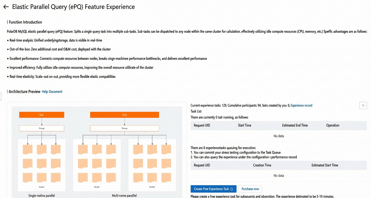
3. At the bottom of the page, click the Create Free Trial Task button.

4. After a moment, click to refresh the task list. The trial task that you created appears in the list.

5. Click View Details to go to the real-time query trial page.

6. First, perform a Normal Query task without ePQ enabled.

   Note

   Follow the on-screen prompts and click the buttons to perform each step. If you do not click a button before the countdown ends, the operation runs automatically.

   1. Click the Start Task button to begin the trial.

   2. Click the Configure Query Database button. The following command is automatically run on the PolarDB cluster to switch to the tpch database:

      use tpch;

   3. Click the Configure Parallel Policy to LOCAL button. The following command is automatically run to set the database's parallel policy to LOCAL:

      set parallel_workers_policy='LOCAL' ;

   4. Click the Configure Parallelism to 0 button. The following command is automatically run to set the degree of parallelism to 0.

      set max_parallel_degree=0;

   5. Click the View Execution Plan button. The following command is automatically run to view the execution plan for the following SQL statement.

      explain format=TREE  SELECT SUM(p_retailprice), AVG(p_retailprice)
          ->  , MIN(p_retailprice), MAX(p_retailprice)
          -> FROM part
          -> GROUP BY p_type
          -> ORDER BY 1
          -> LIMIT 1;

      The execution plan is as follows:

      +------------------------------------------------------------------------------+
      | EXPLAIN                                                                                                                                                                                                                                                       |
      +------------------------------------------------------------------------------+
      | -> Limit: 1 row(s)
          -> Sort: <temporary>.sum(p_retailprice), limit input to 1 row(s) per chunk
              -> Table scan on <temporary>
                  -> Aggregate using temporary table
                      -> Table scan on part  (cost=2123689.64 rows=19896680)
       |
      +------------------------------------------------------------------------------+
      1 row in set (0.00 sec)

      In a normal query plan, the table scan and aggregation are performed serially in a single thread.

   6. Click the Execute SQL button. The SQL statement from the previous step is automatically run:

      SELECT SUM(p_retailprice), AVG(p_retailprice)
          ->  , MIN(p_retailprice), MAX(p_retailprice)
          -> FROM part
          -> GROUP BY p_type
          -> ORDER BY 1
          -> LIMIT 1;

      The following result is returned. The running time is 22.47 seconds.

      +--------------------+--------------------+--------------------+--------------------+
      | SUM(p_retailprice) | AVG(p_retailprice) | MIN(p_retailprice) | MAX(p_retailprice) |
      +--------------------+--------------------+--------------------+--------------------+
      |       198461679.87 |        1498.366804 |             901.47 |            2098.51 |
      +--------------------+--------------------+--------------------+--------------------+
      1 row in set (22.47 sec)

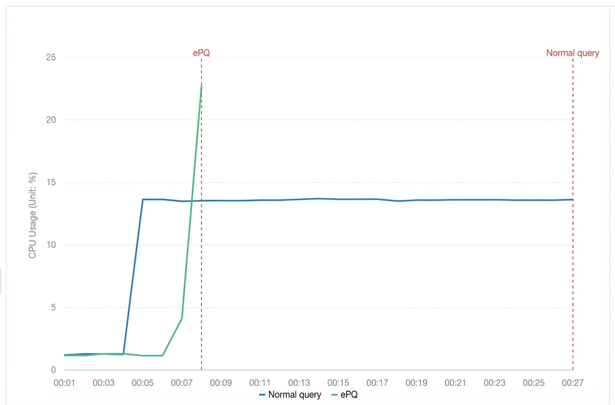
   7. During this process, observe the changes in the average cluster CPU utilization in the trend graph on the left.

7. After the normal query is complete, the task automatically switches to the ePQ Query task. Follow the on-screen prompts and click the buttons to perform each step. If you do not click a button before the countdown ends, the operation runs automatically.

   1. Click the Configure Cross-Node Parallel Query button. The following command is automatically run to enable the ePQ feature.

      set parallel_workers_policy='MULTI_NODES';

   2. Click the Configure Parallelism to 4 button. The following command is automatically run to set the degree of parallelism for ePQ to 4.

      set max_parallel_degree=4;

   3. Click the View Execution Plan button. The following command is automatically run to view the execution plan for the same SQL statement.

      explain format=TREE SELECT SUM(p_retailprice), AVG(p_retailprice)
          ->  , MIN(p_retailprice), MAX(p_retailprice)
          -> FROM part
          -> GROUP BY p_type
          -> ORDER BY 1
          -> LIMIT 1;

      The execution plan is as follows:

      +-----------------------------------------------------------------------------------------------------------------------------------+
      | EXPLAIN                                                                                                                           |
      +-----------------------------------------------------------------------------------------------------------------------------------+
      | -> Limit: 1 row(s)  (cost=2026377.94 rows=1)
          -> Gather (merge sort; slice: 1; workers: 8; nodes: 2)  (cost=2026377.94 rows=8)
              -> Limit: 1 row(s)  (cost=2026366.65 rows=1)
                  -> Sort: <temporary>.sum(p_retailprice), limit input to 1 row(s) per chunk  (cost=2026366.65 rows=248708)
                      -> Table scan on <temporary>
                          -> Aggregate using temporary table  (cost=2026366.65 rows=248708)
                              -> Repartition (hash keys: part.p_type; slice: 2; workers: 8; nodes: 2)  (cost=1767690.54 rows=248709)
                                  -> Table scan on <temporary>
                                      -> Aggregate using temporary table  (cost=1732861.35 rows=248708)
                                          -> Parallel table scan on part, with parallel partitions: 798  (cost=265461.20 rows=2487085)
       |
      +-----------------------------------------------------------------------------------------------------------------------------------+
      1 row in set (0.00 sec)

      In the query plan with ePQ, the table scan and aggregation are pushed down to eight worker threads across two nodes for concurrent computing.

   4. Click the Execute SQL button. The SQL statement is automatically run:

      SELECT SUM(p_retailprice), AVG(p_retailprice)
          ->  , MIN(p_retailprice), MAX(p_retailprice)
          -> FROM part
          -> GROUP BY p_type
          -> ORDER BY 1
          -> LIMIT 1;

      The following result is returned. The running time is 2.82 seconds.

      +--------------------+--------------------+--------------------+--------------------+
      | SUM(p_retailprice) | AVG(p_retailprice) | MIN(p_retailprice) | MAX(p_retailprice) |
      +--------------------+--------------------+--------------------+--------------------+
      |       198461679.87 |        1498.366804 |             901.47 |            2098.51 |
      +--------------------+--------------------+--------------------+--------------------+
      1 row in set (2.82 sec)

   5. While the SQL statement runs, observe the changes in the average cluster CPU utilization in the trend graph on the left.

      Note

      Real-time monitoring data may be delayed. To ensure that the complete change in CPU utilization is displayed, the trend graph automatically extends the monitoring time by 2 to 3 seconds after the SQL statement finishes.

8. (Optional) To view the results of created tasks, on the Elastic Parallel Query (ePQ) page, click Trial Records. In the panel that appears, click All Tasks or My Tasks to view the details of the trial results.

Result analysis

ePQ greatly improves query efficiency

1. In terms of running time, when ePQ is enabled, the running time for the complex query is significantly reduced from 22.47 seconds to 2.82 seconds.

2. In terms of the execution plan, the SQL statement performs a SUM aggregation.

   • In the execution plan for the normal query, the table scan and aggregation are performed serially in a single thread.

   • In the execution plan for the ePQ query, the table scan and aggregation are pushed down to eight worker threads across two nodes for concurrent computing.

ePQ makes full use of idle compute resources and improves overall cluster resource utilization

As shown by the average cluster CPU utilization, the CPU utilization for the ePQ query is higher than for the normal query. This is because when ePQ is enabled, it fully utilizes idle compute resources by allowing idle compute nodes to participate in the computation.

Related topics

• Use Elastic Parallel Query (ePQ)

• Configure parallel resource control policies

• ePQ FAQ

Contact experts

If you have questions or need more technical support, join the official DingTalk group. The DingTalk group number is 12810035247.