This topic provides examples of DataFrame operations in typical scenarios using the SDK for Python.
DataFrame
PyODPS includes a pandas-like API called PyODPS DataFrame, which runs operations directly on MaxCompute for scalable data processing. For more information, see DataFrame.
How PyODPS DataFrame executes operations
PyODPS DataFrame uses lazy evaluation: transformation operations (such as column selection, filtering, and joins) build a query plan but do not submit work to MaxCompute. Execution happens only when you call an action method that retrieves results. Common action methods include:
| Method | Description |
|---|---|
head(n) |
Returns the first n rows |
count() |
Returns the number of rows |
execute() |
Runs the query and returns all results |
persist(table_name) |
Saves the result as a MaxCompute table |
to_pandas() |
Converts the result to a pandas DataFrame |
This distinction matters when reading the examples below: some lines define transformations and others trigger execution.
Prerequisites
Before you begin, make sure you have:
-
A MaxCompute project with permissions to read and write tables
-
PyODPS installed (
pip install pyodps) -
Your AccessKey ID and AccessKey secret stored as environment variables
ALIBABA_CLOUD_ACCESS_KEY_IDandALIBABA_CLOUD_ACCESS_KEY_SECRET
The examples use three tables: pyodps_ml_100k_movies (movie data), pyodps_ml_100k_users (user data), and pyodps_ml_100k_ratings (rating data). These tables must exist in your MaxCompute project before you run the examples. For instructions on loading the MovieLens 100K dataset into MaxCompute, see Bulk load overview.
Connect to MaxCompute and create a DataFrame
-
Create a MaxCompute entry object.
import os from odps import ODPS # Retrieve credentials from environment variables. # Store credentials as environment variables instead of hardcoding them. o = ODPS( os.getenv('ALIBABA_CLOUD_ACCESS_KEY_ID'), os.getenv('ALIBABA_CLOUD_ACCESS_KEY_SECRET'), project='your-default-project', endpoint='your-end-point', ) -
Wrap a MaxCompute table in a DataFrame object.
from odps.df import DataFrame

users = DataFrame(o.get_table('pyodps_ml_100k_users'))
Explore the data
View the schema
Use the dtypes attribute to inspect the fields and their types.
users.dtypesPreview rows
Use head() to fetch the first N rows without downloading the full dataset.
users.head(10)Output:
| - | user_id | age | sex | occupation | zip_code |
|---|---|---|---|---|---|
| 0 | 1 | 24 | M | technician | 85711 |
| 1 | 2 | 53 | F | other | 94043 |
| 2 | 3 | 23 | M | writer | 32067 |
| 3 | 4 | 24 | M | technician | 43537 |
| 4 | 5 | 33 | F | other | 15213 |
| 5 | 6 | 42 | M | executive | 98101 |
| 6 | 7 | 57 | M | administrator | 91344 |
| 7 | 8 | 36 | M | administrator | 05201 |
| 8 | 9 | 29 | M | student | 01002 |
| 9 | 10 | 53 | M | lawyer | 90703 |
Select and transform fields
Select specific fields
Pass a list of field names to return only those columns.
users[['user_id', 'age']].head(5)Output:
| - | user_id | age |
|---|---|---|
| 0 | 1 | 24 |
| 1 | 2 | 53 |
| 2 | 3 | 23 |
| 3 | 4 | 24 |
| 4 | 5 | 33 |
Exclude specific fields
Use exclude() to drop unwanted columns.
users.exclude('zip_code', 'age').head(5)Output:
| - | user_id | sex | occupation |
|---|---|---|---|
| 0 | 1 | M | technician |
| 1 | 2 | F | other |
| 2 | 3 | M | writer |
| 3 | 4 | M | technician |
| 4 | 5 | F | other |
Exclude fields and add a computed column
Combine exclude() with select() to drop columns while adding a derived field. The following example adds sex_bool, which is True when sex is M.
users.select(users.exclude('zip_code', 'sex'), sex_bool=users.sex == 'M').head(5)Output:
| - | user_id | age | occupation | sex_bool |
|---|---|---|---|---|
| 0 | 1 | 24 | technician | True |
| 1 | 2 | 53 | other | False |
| 2 | 3 | 23 | writer | True |
| 3 | 4 | 24 | technician | True |
| 4 | 5 | 33 | other | False |
Aggregate and analyze
Count rows matching a condition
users.age.between(20, 25).count().rename('count')Output:
943Group by a field
Count users by sex.
users.groupby(users.sex).count()Output:
| - | sex | count |
|---|---|---|
| 0 | F | 273 |
| 1 | M | 670 |
Top 10 occupations by user count
Chain groupby, agg, and sort to rank occupations in descending order. Each method returns a new DataFrame, so you can continue chaining; the slice [:10] triggers execution and retrieves results.
df = users.groupby('occupation').agg(count=users['occupation'].count())
df.sort(df['count'], ascending=False)[:10]
Output:
| - | occupation | count |
|---|---|---|
| 0 | student | 196 |
| 1 | other | 105 |
| 2 | educator | 95 |
| 3 | administrator | 79 |
| 4 | engineer | 67 |
| 5 | programmer | 66 |
| 6 | librarian | 51 |
| 7 | writer | 45 |
| 8 | executive | 32 |
| 9 | scientist | 31 |
value_counts() produces the same result with less code:
users.occupation.value_counts()[:10]Visualize data
Enable inline plotting in Jupyter Notebook before drawing charts.
%matplotlib inlineHorizontal bar chart
Plot occupation counts as a horizontal bar chart.
users['occupation'].value_counts().plot(kind='barh', x='occupation', ylabel='prefession')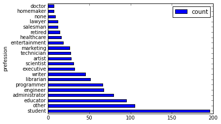
Histogram
Divide users into 30 age bins and plot the distribution.
users.age.hist(bins=30, title="Distribution of users' ages", xlabel='age', ylabel='count of users')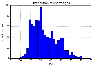
Join tables and persist results
Load all three tables, join them, and save the result as a new MaxCompute table.
movies = DataFrame(o.get_table('pyodps_ml_100k_movies'))
ratings = DataFrame(o.get_table('pyodps_ml_100k_ratings'))

o.delete_table('pyodps_ml_100k_lens', if_exists=True)
lens = movies.join(ratings).join(users).persist('pyodps_ml_100k_lens')
lens.dtypes
Output:
odps.Schema {
  movie_id                            int64
  title                               string
  release_date                        string
  video_release_date                  string
  imdb_url                            string
  user_id                             int64
  rating                              int64
  unix_timestamp                      int64
  age                                 int64
  sex                                 string
  occupation                          string
  zip_code                            string
}
Analyze ratings by age group
Create age groups
Use cut() to assign each row to a decade-based age group.
labels = ['0-9', '10-19', '20-29', '30-39', '40-49', '50-59', '60-69', '70-79']
cut_lens = lens[lens, lens.age.cut(range(0, 80, 10), right=False, labels=labels).rename('age_group')]
Inspect the grouping
Verify the age-to-group mapping by viewing the first 10 distinct combinations.
cut_lens['age_group', 'age'].distinct()[:10]Output:
| - | age_group | age |
|---|---|---|
| 0 | 0-9 | 7 |
| 1 | 10-19 | 10 |
| 2 | 10-19 | 11 |
| 3 | 10-19 | 13 |
| 4 | 10-19 | 14 |
| 5 | 10-19 | 15 |
| 6 | 10-19 | 16 |
| 7 | 10-19 | 17 |
| 8 | 10-19 | 18 |
| 9 | 10-19 | 19 |
Total and average rating per age group
cut_lens.groupby('age_group').agg(
    cut_lens.rating.count().rename('total_rating'),
    cut_lens.rating.mean().rename('average_rating')
)
Output:
| - | age_group | average_rating | total_rating |
|---|---|---|---|
| 0 | 0-9 | 3.767442 | 43 |
| 1 | 10-19 | 3.486126 | 8181 |
| 2 | 20-29 | 3.467333 | 39535 |
| 3 | 30-39 | 3.554444 | 25696 |
| 4 | 40-49 | 3.591772 | 15021 |
| 5 | 50-59 | 3.635800 | 8704 |
| 6 | 60-69 | 3.648875 | 2623 |
| 7 | 70-79 | 3.649746 | 197 |