Quickly deploy an inference service based on the DeepSeek model-Object Storage Service(OSS)-阿里云帮助中心

Advantages of OSS in AI scenarios

Advantage	Description
High throughput and high concurrency	The distributed architecture allows business data to be distributed across multiple data clusters as needed. This enables parallel processing of large-scale data read and write requests. Stateless access endpoints support large-scale horizontal scaling. This significantly improves the system's concurrent processing capabilities and access bandwidth.
Low-cost tiered storage	The object versioning feature automatically saves different versions of the same object. This ensures that model and data versions are traceable and supports safe iterations. Multiple lifecycle management policies automate tiered storage. This reduces long-term data retention costs.
High reliability	99.9999999999% (12 nines) of data durability prevents AI training tasks from being interrupted or data from being lost due to storage failures. 99.995% data availability provides stable read and write services. This ensures the stable operation of AI services such as online inference.
Efficient distribution and sharing	Natively suited for distributed access and large-scale content delivery. This improves the deployment efficiency of inference nodes. Multiple fine-grained authorization policies enable efficient and secure sharing of AI data.

Load large models in seconds via OSS Connector for AI/ML

OSS Connector for AI/ML is designed to improve model loading and data access efficiency for AI inference. You can integrate it seamlessly without changing your inference framework. Its core advantages include the following:

Out-of-the-box: Seamlessly integrates with mainstream frameworks without code modification.
Load 100 GB models in seconds: User-mode I/O acceleration delivers performance several times higher than Filesystem in Userspace (FUSE).
100% bandwidth utilization: A self-developed high-concurrency network module fully utilizes OSS throughput.
Smart prefetch cache: Preloads hot data in memory to significantly reduce inference latency.

Achieve optimal performance on a single node

Step 1: Build a high-performance computing and elastic network environment

On the Elastic Compute Service (ECS) instances page, create an ECS instance.

This tutorial uses an ecs.g8i.48xlarge instance as an example. This instance provides a 192-core CPU, 1 TiB of memory, and a base network bandwidth of 100 Gbit/s. This ensures sufficient computing resources and network bandwidth to support AI/ML tasks and OSS data transmission requirements.
Create an elastic network interface on the ENIs page. The Elastic Network Interface (ENI) must be in the same virtual private cloud (VPC) as the ECS instance.

You can aggregate bandwidth from multiple ENIs to achieve high-throughput access to OSS within the VPC, which overcomes the bandwidth limit of a single ENI.
Associate the ENI with the ECS instance that you created.

View the ENI information.

The two local routing entries local 172.16.6.121 dev eth0 and local 172.16.6.122 dev eth1 indicate that both ENIs have successfully obtained IP addresses.

(xxx                              ]# ip link show
1: lo: <LOOPBACK,UP,LOWER_UP> mtu 65536 qdisc noqueue state UNKNOWN mode DEFAULT group default qlen 1000
    link/loopback 00:00:00:00:00:00 brd 00:00:00:00:00:00
2: eth0: <BROADCAST,MULTICAST,UP,LOWER_UP> mtu 8500 qdisc mq state UP mode DEFAULT group default qlen 1000
    link/ether xxx brd ff:ff:ff:ff:ff:ff
    altname enp2s1
3: eth1: <BROADCAST,MULTICAST,UP,LOWER_UP> mtu 8500 qdisc mq state UP mode DEFAULT group default qlen 1000
    link/ether xxx brd ff:ff:ff:ff:ff:ff
    altname enp7s2
(xxx                              ]# ip route show table local
broadcast 127.0.0.0 dev lo proto kernel scope link src 127.0.0.1
local 127.0.0.0/8 dev lo proto kernel scope host src 127.0.0.1
local 127.0.0.1 dev lo proto kernel scope host src 127.0.0.1
broadcast 127.255.255.255 dev lo proto kernel scope link src 127.0.0.1
broadcast 172.16.6.0 dev eth0 proto kernel scope link src 172.16.6.121
broadcast 172.16.6.0 dev eth1 proto kernel scope link src 172.16.6.122
local 172.16.6.121 dev eth0 proto kernel scope host src 172.16.6.121
local 172.16.6.122 dev eth1 proto kernel scope host src 172.16.6.122
broadcast 172.16.6.255 dev eth0 proto kernel scope link src 172.16.6.121
broadcast 172.16.6.255 dev eth1 proto kernel scope link src 172.16.6.122
(xxx                              ]# ip route show table main
default via 172.16.6.253 dev eth0 proto dhcp src 172.16.6.121 metric 100
default via 172.16.6.253 dev eth1 proto dhcp src 172.16.6.122 metric 101
172.16.6.0/24 dev eth0 proto kernel scope link src 172.16.6.121 metric 100
172.16.6.0/24 dev eth1 proto kernel scope link src 172.16.6.122 metric 101

Step 2: Prepare model data and install the inference framework

Obtain the Q8-quantized, GGUF version of the DeepSeek-R2 model. This model has high inference performance and low memory usage. It is suitable for evaluating the efficiency of large-scale model loading and deployment.
Use ossutil to upload the model file to an OSS bucket in the same region through an internal endpoint.
Use llama.cpp as the inference framework. It supports efficient loading and running of models in GGUF format.
1. Clone the llama.cpp repository from GitHub to your local machine.
```
git clone https://github.com/ggerganov/llama.cpp
```
2. Go to the project directory.
```
cd llama.cpp
```
3. Create a build directory.
```
mkdir build
```
4. Generate the build configuration.
```
cmake -B build -DCMAKE_BUILD_TYPE=Release
```
5. Compile the project.
```
cmake --build build --config Release
```

Step 3: Install OSS Connector and start the inference service

Install and configure OSS Connector.

Download the installation package.

wget https://gosspublic.alicdn.com/oss-connector/oss-connector-lib-1.1.0rc7.x86_64.rpm

Install OSS Connector.

yum install -y oss-connector-lib-1.1.0rc7.x86_64.rpm

Configure OSS Connector.

Modify the configuration file in the /etc/oss-connector/config.json path.

{
    "logLevel": 1,
    "logPath": "/var/log/oss-connector/connector.log",
    "auditPath": "/var/log/oss-connector/audit.log",
    "expireTimeSec": 120,
    "prefetch": {
        "vcpus": 32,
        "workers": 32
    }
}

Set the environment variables.

export OSS_ACCESS_KEY_ID=LTA********
export OSS_ACCESS_KEY_SECRET=tg********
export OSS_REGION=cn-beijing
export OSS_ENDPOINT=oss-cn-beijing-internal.aliyuncs.com
export OSS_PATH=oss://<BUCKET-NAME>/deepseek/DeepSeek-R2-Q8_0/
export MODEL_DIR=/tmp/model/DeepSeek-R2-Q8_0/
export HTTP_SOURCE_IP=172.xx.x.xxx,172.xx.x.xxx

Environment variable key	Description
OSS_ACCESS_KEY_ID	The AccessKey ID and AccessKey secret of an Alibaba Cloud account or a Resource Access Management (RAM) user. When you use a temporary access credential from STS, set these variables to the AccessKey ID and AccessKey secret of the credential. To use OSS Connector, you need the oss:ListObjects permission for the target bucket directory. If the bucket and files you want to access support anonymous access, you can leave the OSS_ACCESS_KEY_ID and OSS_ACCESS_KEY_SECRET environment variables unset or set them to empty strings.
OSS_ACCESS_KEY_SECRET
OSS_SESSION_TOKEN	The temporary access token. You must set this parameter when you use a temporary access credential obtained from Security Token Service (STS) to access OSS. When you use the AccessKey pair of an Alibaba Cloud account or a RAM user, leave this field empty.
OSS_ENDPOINT	Specifies the OSS service endpoint. Example: `http://oss-cn-beijing-internal.aliyuncs.com`. If you do not specify a protocol, HTTPS is used by default. We recommend that you use HTTP in secure environments, such as an internal network, for better performance.
OSS_REGION	Specifies the OSS Region ID. Example: cn-beijing. If this is not specified, authentication may fail.
OSS_PATH	The OSS path for the model must be in the oss://bucketname/path/ format. For example: `oss://examplebucket/deepseek/DeepSeek-R2-Q8_0/`.
MODEL_DIR	The local path of the model. Example: `/tmp/model/DeepSeek-R2-Q8_0/`.
HTTP_SOURCE_IP	Specifies the IP addresses of the ENIs for the connector to use. Obtain these IP addresses following instructions in the ENI information section. (Examples: 172.16.6.121 and 172.16.6.122). Linux automatically selects the corresponding network interfaces (such as eth0 and eth1) and routes traffic based on these IP addresses. For more fine-grained routing control, such as traffic splitting by source IP or destination address, you can use `ip rule` with custom route tables to configure policy-based routing.

Start the inference service.

LD_PRELOAD=/usr/local/lib/libossc_preload.so ENABLE_CONNECTOR=1 llama-server -m /tmp/model/DeepSeek-R2-Q8_0/DeepSeek-R2.Q8_0-00001-of-00015.gguf -t 48 -c 1024 --host 0.0.0.0 --port 9090 --numa isolate

Step 4: Observe performance

After the inference service starts, the internal network bandwidth of the ECS instance changes as follows within one minute:

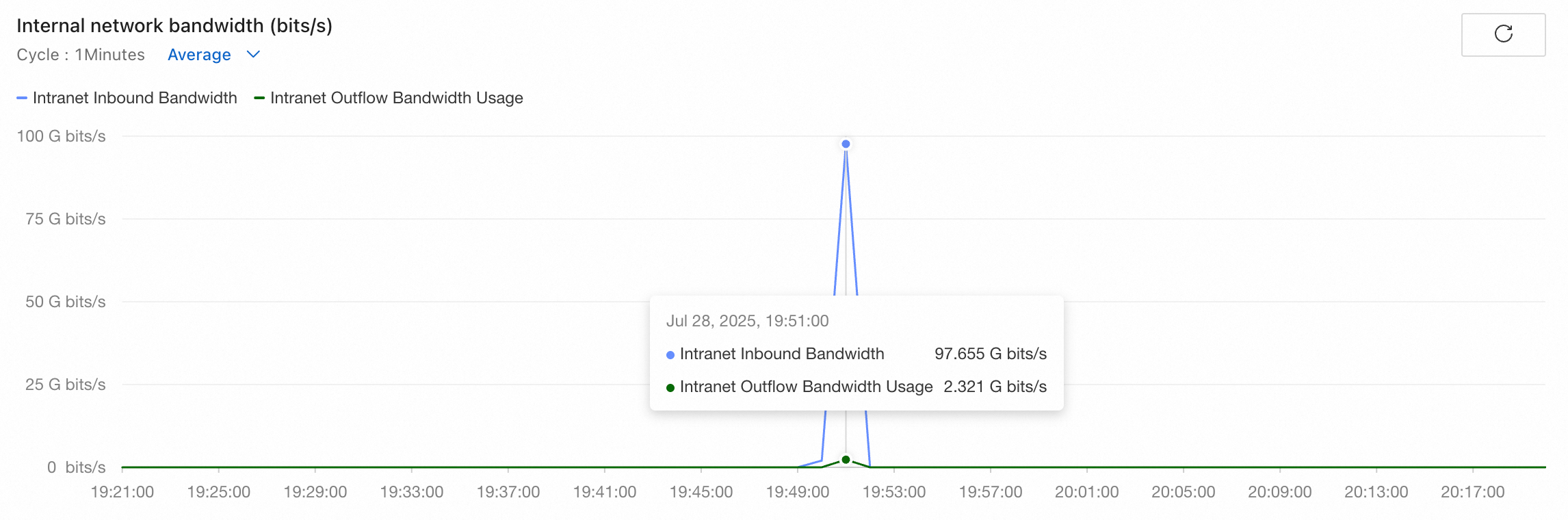
The network traffic on the ECS instance shows that the combined baseline bandwidth of the dual ENIs is continuously saturated at 100 Gbit/s:

31s      IFACE   rxpck/s   txpck/s    rxkB/s    txkB/s   rxcmp/s   txcmp/s  rxmcst/s   %ifutil
32s         lo      0.00      0.00      0.00      0.00      0.00      0.00      0.00      0.00
32s       eth0 4685527.00 2914154.00 6576352.14 233729.15      0.00      0.00      0.00      0.00
32s       eth1 4431023.00      0.00 6219142.01      0.00      0.00      0.00      0.00      0.00

32s      IFACE   rxpck/s   txpck/s    rxkB/s    txkB/s   rxcmp/s   txcmp/s  rxmcst/s   %ifutil
33s         lo      0.00      0.00      0.00      0.00      0.00      0.00      0.00      0.00
33s       eth0 4643666.00 2968261.00 6517694.15 238021.36      0.00      0.00      0.00      0.00
33s       eth1 4472967.00      0.00 6278001.55      0.00      0.00      0.00      0.00      0.00

33s      IFACE   rxpck/s   txpck/s    rxkB/s    txkB/s   rxcmp/s   txcmp/s  rxmcst/s   %ifutil
34s         lo      0.00      0.00      0.00      0.00      0.00      0.00      0.00      0.00
34s       eth0 4698994.00 3100866.00 6595290.37 250645.66      0.00      0.00      0.00      0.00
34s       eth1 4417638.00      0.00 6200418.34      0.00      0.00      0.00      0.00      0.00

34s      IFACE   rxpck/s   txpck/s    rxkB/s    txkB/s   rxcmp/s   txcmp/s  rxmcst/s   %ifutil
35s         lo      0.00      0.00      0.00      0.00      0.00      0.00      0.00      0.00
35s       eth0 4673228.00 2882323.00 6559128.50 229996.60      0.00      0.00      0.00      0.00
35s       eth1 4443430.00      1.00 6236539.08      0.04      0.00      0.00      0.00      0.00

35s      IFACE   rxpck/s   txpck/s    rxkB/s    txkB/s   rxcmp/s   txcmp/s  rxmcst/s   %ifutil
36s         lo      0.00      0.00      0.00      0.00      0.00      0.00      0.00      0.00
36s       eth0 4706184.00 2963548.00 6605398.16 237661.12      0.00      0.00      0.00      0.00
36s       eth1 4410386.00      0.00 6190296.66      0.00      0.00      0.00      0.00      0.00

36s      IFACE   rxpck/s   txpck/s    rxkB/s    txkB/s   rxcmp/s   txcmp/s  rxmcst/s   %ifutil
37s         lo      0.00      0.00      0.00      0.00      0.00      0.00      0.00      0.00
37s       eth0 4723438.00 2932274.00 6629798.87 235513.98      0.00      0.00      0.00      0.00
37s       eth1 4392835.00      0.00 6165661.72      0.00      0.00      0.00      0.00      0.00

The following table shows the actual statistics from this test and compares them with other loading solutions such as ossfs.

Loading tool	End-to-end startup time for the inference service (includes OSS access and model loading)	OSS single-account bandwidth limit	Actual bandwidth used	Total data read from OSS
OSS Connector for AI/ML	81s	100 Gbit/s	100 Gbit/s	664 GB
ossfs 2.0	257s	100 Gbit/s	20 Gbit/s	666 GB
ossfs 1.0	1020s	100 Gbit/s	6.4 Gbit/s	782 GB

Deployment solution for large-scale inference nodes

Accelerate the startup of large-scale inference nodes with a P2P solution

OSS Connector for AI/ML can work with a self-developed peer-to-peer (P2P) distribution system to efficiently share and transfer the same model data among multiple nodes. This P2P system is designed for typical inference deployment scenarios where multiple nodes load the same data simultaneously. It significantly reduces the access pressure on the central data source (OSS) and improves overall bandwidth utilization. The system supports an on-demand distribution mechanism and can perform random and streaming reads of large files. It prioritizes reducing the access latency of individual data fragments while ensuring accuracy. Additionally, the underlying design supports high-concurrency access, meeting the requirements of large-scale inference tasks for both distribution efficiency and stability.

Effective peak shaving and throttling: By sharing data between nodes, the system significantly reduces the load on OSS bandwidth during the concurrent startup of many inference nodes. This greatly reduces the instantaneous pressure on the central data source.
Sustained high performance: The system relies on the connector to pull raw data from OSS, fully leveraging the connector's performance to ensure low latency and high throughput for initial data access.
Native support for horizontal scaling: The system supports large-scale horizontal scaling of inference nodes and provides excellent concurrent startup capabilities. Even in a cluster with hundreds of nodes, the startup time is similar to that of a single node.
Significant reduction in back-to-origin traffic: Through local caching and the P2P distribution mechanism, the system minimizes repeated data pulls. This effectively controls the back-to-origin traffic of OSS and improves overall resource utilization efficiency.

Test environment and method

Use the Q8 quantized version of the DeepSeek-R2 model in GGUF format, with a total size of 664 GB. The inference framework is llama.cpp.
Use 50 ecs.g8i.48xlarge ECS instances to build an inference cluster. This test uses Container Service for Kubernetes (ACK) to manage and deploy the inference cluster. The inference service runs as the main process in a container, ensuring efficient and stable service startup. This enables flexible scheduling and resource management in a containerized environment.
The startup log timestamp of the llama.cpp inference framework is used as a reference point to determine when model loading is complete. This measures the time from startup until the model is available.
Measurements are taken independently on each inference node. The following key performance indicators (KPIs) are collected: the average and longest loading times for each node, and the total amount of data requested from OSS during the entire deployment process. These metrics provide a comprehensive evaluation of bandwidth utilization efficiency and overall system performance during model loading.

Test results

Average end-to-end startup time for the inference service (includes OSS access and model loading)	OSS single-account bandwidth limit	Total data read from OSS
127s	100 Gbit/s	1262 GB

Conclusion

In this test, the average end-to-end startup time for an inference node was approximately 1.5 times that of a single node. The test results show that even with a significant increase in the number of nodes, the overall deployment time did not increase substantially. Even in a high-concurrency environment, the system maintained stable loading performance and resource scheduling efficiency, demonstrating the solution's excellent horizontal scaling capabilities. Additionally, the total back-to-origin data volume for the entire cluster was only about twice the total model size. This approach effectively controlled the access overhead of the central storage service and significantly reduced the instantaneous bandwidth pressure on the backend storage service caused by concurrent model loading in a large-scale cluster.