Naive Bayes

Component configuration

You can configure the Naive Bayes component parameters in one of the following ways.

Method 1: Designer

Method 2: PAI commands

PAI -name NaiveBayes -project algo_public
    -DinputTablePartitions="pt=20150501"
    -DmodelName="xlab_m_NaiveBayes_23772"
    -DlabelColName="poutcome"
    -DfeatureColNames="age,previous,cons_conf_idx,euribor3m"
    -DinputTableName="bank_data_partition";

Example

1. Prepare the training data and test data.

   1. Use the MaxCompute client to create the train_data and test_data tables to store the training and test data, respectively. Both tables must have the following column names and data types: id bigint, y bigint, f0 double, f1 double, f2 double, f3 double, f4 double, f5 double, f6 double, f7 double. For instructions on installing and configuring the MaxCompute client, see MaxCompute client (odpscmd). For instructions on creating a table, see Create tables.

   2. Import the following training and test data into the train_data and test_data tables, respectively. For instructions on importing data, see Import data.

      • Training data

        id	y	f0	f1	f2	f3	f4	f5	f6	f7
        1	-1	-0.294118	0.487437	0.180328	-0.292929	-1	0.00149028	-0.53117	-0.0333333
        2	+1	-0.882353	-0.145729	0.0819672	-0.414141	-1	-0.207153	-0.766866	-0.666667
        3	-1	-0.0588235	0.839196	0.0491803	-1	-1	-0.305514	-0.492741	-0.633333
        4	+1	-0.882353	-0.105528	0.0819672	-0.535354	-0.777778	-0.162444	-0.923997	-1
        5	-1	-1	0.376884	-0.344262	-0.292929	-0.602837	0.28465	0.887276	-0.6
        6	+1	-0.411765	0.165829	0.213115	-1	-1	-0.23696	-0.894962	-0.7
        7	-1	-0.647059	-0.21608	-0.180328	-0.353535	-0.791962	-0.0760059	-0.854825	-0.833333
        8	+1	0.176471	0.155779	-1	-1	-1	0.052161	-0.952178	-0.733333
        9	-1	-0.764706	0.979899	0.147541	-0.0909091	0.283688	-0.0909091	-0.931682	0.0666667
        10	-1	-0.0588235	0.256281	0.57377	-1	-1	-1	-0.868488	0.1

      • Test data

        id	y	f0	f1	f2	f3	f4	f5	f6	f7
        1	+1	-0.882353	0.0854271	0.442623	-0.616162	-1	-0.19225	-0.725021	-0.9
        2	+1	-0.294118	-0.0351759	-1	-1	-1	-0.293592	-0.904355	-0.766667
        3	+1	-0.882353	0.246231	0.213115	-0.272727	-1	-0.171386	-0.981213	-0.7
        4	-1	-0.176471	0.507538	0.278689	-0.414141	-0.702128	0.0491804	-0.475662	0.1
        5	-1	-0.529412	0.839196	-1	-1	-1	-0.153502	-0.885568	-0.5
        6	+1	-0.882353	0.246231	-0.0163934	-0.353535	-1	0.0670641	-0.627669	-1
        7	-1	-0.882353	0.819095	0.278689	-0.151515	-0.307329	0.19225	0.00768574	-0.966667
        8	+1	-0.882353	-0.0753769	0.0163934	-0.494949	-0.903073	-0.418778	-0.654996	-0.866667
        9	+1	-1	0.527638	0.344262	-0.212121	-0.356974	0.23696	-0.836038	-0.8
        10	+1	-0.882353	0.115578	0.0163934	-0.737374	-0.56974	-0.28465	-0.948762	-0.933333

2. Build and run the pipeline by following these steps. For more information, see algorithm modeling.

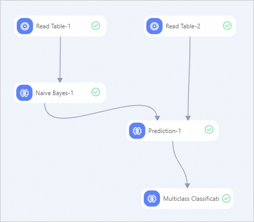
   1. From the component list in Designer, drag the following components onto the canvas: two Read Table components, one Naive Bayes component, one Prediction component, and one Multiclass Classification Evaluation component.

   2. Connect the nodes to build the pipeline.

   3. Configure the component parameters.

      • Click the Read Table-1 component on the canvas. In the right-side pane, on the select table tab, set table name to train_data.

      • Click the Read Table-2 component on the canvas. In the right-side pane, on the select table tab, set table name to test_data.

      • Click the Naive Bayes-1 component on the canvas. In the right-side pane, set the parameters as follows. Leave the other parameters at their default values.

        Tab	Parameter	Description
        field settings	feature column	Select the f0, f1, f2, f3, f4, f5, f6, and f7 columns.
        	label column	Select the y column.

      • Click the Prediction-1 component on the canvas. In the right-side pane, on the field settings tab, set reserved columns to id and y. Leave the other parameters at their default values.

      • Click the Multiclass Classification Evaluation-1 component on the canvas. In the right-side pane, on the field settings tab, set original classification result column to y. Leave the other parameters at their default values.

   4. Once the components are configured, click the Run button to run the pipeline.

3. After the pipeline runs, right-click the Prediction-1 component and select View Data > Prediction Result Output from the shortcut menu. The prediction result table contains the id, y (original label), prediction_result (prediction label, with a value of 1 or -1), prediction_score (prediction score), and prediction_detail (class probability details in JSON format) columns. For the 10 test samples, the prediction scores are close to 1, indicating high model confidence and good performance.