Scorecard training

Scorecard Training involves the following concepts:

• Feature engineering

  The primary difference between a scorecard model and a standard linear model is the feature engineering process applied to the data before training. The Scorecard Training component offers two feature engineering methods:

  • Use the Binning component to discretize features. Then, apply one-hot encoding to each variable based on the binning results to generate N dummy variables, where N is the number of bins for the variable.

    Note

    When you use dummy variable transformation, you can set constraints between the dummy variables of each original variable. For more information, see Binning.

  • Use the Binning component to discretize features, and then perform a Weight of Evidence (WOE) conversion. This replaces the original value of a variable with the WOE value of the bin into which the variable falls.

• Score transformation

  In credit scoring, a linear transformation converts the predicted sample odds into a score. This transformation typically uses the following formula.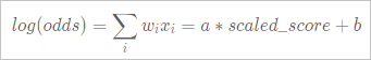You can specify the linear transformation by using the following three parameters:

  • scaledValue: A baseline score.

  • odds: The odds value at the specified baseline score.

  • pdo (Points to Double Odds): The number of points by which the score must increase for the odds value to double.

  For example, if scaledValue=800, odds=50, and pdo=25, two points on the line are defined as follows:

  log(50)=a×800+b
  log(100)=a×825+b

  By solving for a and b, you can apply the linear transformation to the model's scores to get the final variable scores.

  Specify the scaling information in JSON format using the -Dscale parameter, as shown in the following example.

  {"scaledValue":800,"odds":50,"pdo":25}

  If the -Dscale parameter is not empty, you must specify values for scaledValue, odds, and pdo.

• Training constraints

  Scorecard Training supports adding constraints to variables. For example, you can set the score for a specific bin to a fixed value, enforce a proportional relationship between the scores of two bins, limit the range of scores between bins, or order bin scores according to their WOE values. The underlying constrained optimization algorithm implements these constraints. You can configure constraints visually in the Binning component, which then generates a JSON-formatted condition and automatically passes it to the downstream training component. In the parameter settings panel for the Binning node of your scorecard experiment, set the Feature Columns (supports STRING, BIGINT, and DOUBLE types), Label Column (value is class), and Positive Label to 1. Then, select the Custom JSON File for Binning option and upload your constraint file (for example, binning.txt). The constraint JSON is stored as a string in a single-row, single-column table. The system supports the following six types of JSON constraints:

  • "<": Enforces that the variable weights are in ascending order.

  • ">": Enforces that the variable weights are in descending order.

  • "=": Sets a variable weight to a fixed value.

  • "%": Enforces a proportional relationship between variable weights.

  • "UP": Sets an upper bound for a variable's weight. For example, a value of 0.5 means the trained weight cannot exceed 0.5.

  • "LO": Sets a lower bound for a variable's weight. For example, a value of 0.5 means the trained weight must be at least 0.5.

  This table must contain a single column of the STRING type. The following code shows a sample JSON string.

  {
      "name": "feature0",
      "<": [
          [0,1,2,3]
      ],
      ">": [
          [4,5,6]
      ],
      "=": [
          "3:0","4:0.25"
      ],
      "%": [
          ["6:1.0","7:1.0"]
      ]
  }

• Built-in constraints

  Each original variable has an implicit constraint that you do not need to specify: the average score for a single variable across the population is zero. Because of this constraint, the scaled_weight of the model's intercept represents the average score of the entire population.

• Optimization algorithms

  You can configure the optimization algorithm in the advanced options. The system supports the following four optimization algorithms:

  • L-BFGS: A first-order optimization algorithm that supports large-scale feature datasets. This is an unconstrained optimization algorithm and automatically ignores any specified constraints.

  • Newton's method: A classic second-order algorithm known for fast convergence and high accuracy. However, it is not suitable for large-scale features because it requires computing a second-order Hessian matrix. This is also an unconstrained optimization algorithm and ignores any specified constraints.

  • Barrier method: A second-order optimization algorithm. Without constraints, it is identical to Newton's method. Its computational performance and accuracy are similar to SQP.

  • SQP

    SQP is a second-order optimization algorithm that supports constraints. Without constraints, it is identical to Newton's method. We generally recommend using SQP, as its performance is similar to the barrier method.

  Note

  • L-BFGS and Newton's method are unconstrained optimization algorithms. The barrier method and SQP are constrained optimization algorithms.

  • If you are not familiar with optimization algorithms, we recommend setting the optimization algorithm to Auto Selection. The system automatically chooses the most suitable algorithm based on your data size and constraints.

• Feature selection

  The training component supports stepwise feature selection. This method combines forward selection and backward elimination. Each time a new variable is added to the model through forward selection, the system performs a backward elimination step on all variables already in the model to remove any that no longer meet the significance requirement. Because it supports multiple objective functions and feature transformation methods, the stepwise process supports the following selection criteria:

  • Marginal contribution: Applicable to all objective functions and feature engineering methods.

    The marginal contribution of a variable X is the difference between the objective function values of two models at convergence: Model A (which does not include X) and Model B (which includes all variables from A plus X). When you use dummy variable transformation, the marginal contribution of the original variable X is defined as the difference in the objective function between two models: one including all dummy variables for X and one without. Therefore, using marginal contribution for feature selection is compatible with all feature engineering methods.

    The advantage of this method is its flexibility. It is not limited to a specific model type and directly selects variables that improve the objective function. The disadvantage is that, unlike statistical significance where a p-value of 0.05 is a common threshold, marginal contribution does not have a universally accepted threshold. For new users, we recommend starting with a threshold of 10E-5.

  • Score test: Supports only logistic regression with WOE conversion or without feature engineering.

    In the forward selection process, a model with only an intercept is trained first. In each subsequent step, it calculates the score chi-square statistic for each variable not yet in the model. The variable with the largest score chi-square is added to the model. The process then calculates a p-value corresponding to this statistic based on the chi-square distribution. If the p-value of the best variable is greater than the specified entry threshold (slentry), the variable is not added, and the selection process stops.

    After a round of forward selection, a backward elimination round is performed on the variables already in the model. During backward elimination, the process calculates the Wald chi-square statistic and its corresponding p-value for each variable in the model. If a variable's p-value exceeds the specified removal threshold (slstay), it is removed from the model, and the process continues to the next iteration.

  • F test: Supports only linear regression with WOE conversion or without feature engineering.

    In the forward selection process, a model with only an intercept is trained first. In each subsequent step, the F-value is calculated for each variable not yet in the model. Calculating the F-value is similar to calculating marginal contribution, as it requires training two models. The F-value follows an F-distribution, and its corresponding p-value can be derived from its probability density function. If a variable's p-value exceeds the specified entry threshold (slentry), it is not added to the model, and the process stops.

    The backward elimination process also uses the F-value to calculate significance, much like the score test.

• Forced variables

  Before feature selection begins, you can force certain variables into the model. These variables are excluded from the forward and backward selection processes and are included in the final model regardless of their significance. You can use the -Dselected parameter in the command line to specify the number of iterations and significance thresholds in JSON format. The following code shows an example.

  {"max_step":2, "slentry": 0.0001, "slstay": 0.0001}

  If the -Dselected parameter is empty or max_step is 0, the training process proceeds without feature selection.

You can configure the Scorecard Training component in Machine Learning Designer by using the visual interface (for details, see the Scorecard Training example) or by running a PAI command. The following code shows an example of a PAI command.

pai -name=linear_model -project=algo_public
    -DinputTableName=input_data_table
    -DinputBinTableName=input_bin_table
    -DinputConstraintTableName=input_constraint_table
    -DoutputTableName=output_model_table
    -DlabelColName=label
    -DfeatureColNames=feaname1,feaname2
    -Doptimization=barrier_method
    -Dloss=logistic_regression
    -Dlifecycle=8

The Scorecard Training component outputs a model report that includes binning information, bin constraints, and key statistics such as WOE and marginal contribution. The following table describes the columns in the model evaluation report displayed on the PAI web console.

We recommend that you use Machine Learning Designer to submit Scorecard Training jobs. This section describes several example experiments. One example is an experiment named Scorecard Functionality (German Data), which compares scorecard stepwise feature selection, feature WOE conversion, and logistic regression stepwise feature selection. In this workflow, a data source node connects to a Binning node, which then branches to a Scorecard Training-1 node and a Data Transformation-1 node. The Data Transformation-1 node connects to Scorecard Training-2. The two training branches connect to Scorecard Prediction and Scorecard Prediction-2 nodes respectively, which are then followed by evaluation nodes. In the settings for the Scorecard Training-1 node, all columns are selected as features by default (except the label column), the label column is class, and the positive value is 2. The experiment has a deployment status of Not Deployed. Another example is an experiment named Scorecard Test Set Functionality Test. If a test set is connected to the input of the training component, the output model report also includes statistical metrics for the test set, such as WOE and marginal contribution. In this workflow, a data source node connects to a Split node. One output of the Split node connects to a Binning node, which in turn connects to the Scorecard Training node. The second output also connects to the Scorecard Training node. In the component panel, the Finance (beta) section contains components such as Scorecard Training, Scorecard Prediction, Binning, Data Transformation, Score Transformation, and Generalized Linear Regression, which you can drag and drop onto the canvas.