SLB scheduling algorithms

Server Load Balancer (SLB) distributes incoming requests to backend servers based on a scheduling algorithm you configure in each forwarding rule. SLB supports round-robin, weighted round-robin, weighted least connections, and consistent hashing — each suited to different traffic patterns and server configurations.

ALB, NLB, and CLB support different subsets of these algorithms:

• ALB supports weighted round-robin, weighted least connections, and consistent hashing based on source IP addresses and URLs.

• NLB supports round-robin, weighted round-robin, weighted least connections, and consistent hashing based on source IP addresses, the combination of four elements, and QUIC IDs.

• CLB supports round-robin, weighted round-robin, and consistent hashing based on source IP addresses, the combination of four elements, and QUIC IDs.

Round-robin

Overview

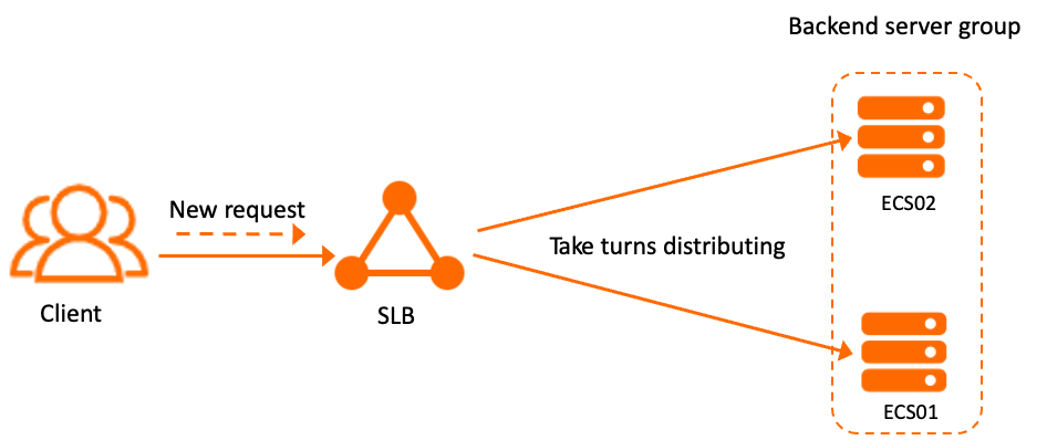
Round-robin distributes requests to backend servers one by one in a fixed sequence. It works well for short-lived, stateless connections like HTTP, where each request is independent and processing time is roughly uniform.

For example, with two Elastic Compute Service (ECS) instances in a backend server group, each instance receives requests alternately — the first request goes to ECS01, the second to ECS02, the third to ECS01, and so on.

Advantages

1. Simple to operate: requires no per-server configuration and is straightforward to set up and maintain.

2. Even distribution: spreads requests evenly across all backend servers when processing time and server capacity are similar.

Disadvantages

1. No real-time load awareness: ignores how busy each server currently is. If server performance varies significantly, faster servers may be underloaded while slower servers become overloaded.

2. Long-lived connections cause imbalance: does not account for connection duration. If some connections stay open much longer than others, those servers accumulate more active connections over time, increasing wait times for subsequent requests.

When to use

1. Uniform server capacity: round-robin performs best when backend servers have similar CPU and memory. With comparable hardware, the even distribution keeps all servers at roughly the same load.

2. Short, stateless requests: a good fit for workloads where each request completes quickly and does not require affinity to a specific server — for example, serving static assets or simple API calls.

Weighted round-robin

Overview

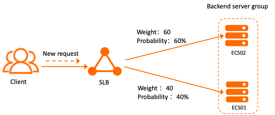
Weighted round-robin extends round-robin by letting you assign a weight to each backend server. Servers with higher weights receive proportionally more requests. Like round-robin, it is well suited to non-consistent connections such as HTTP.

For example, with two ECS instances assigned weights of 60 and 40, the first instance handles 60% of requests and the second handles 40%.

Advantages

1. Proportional distribution: allocates traffic in proportion to each server's weight, so higher-capacity servers carry more of the load without being overwhelmed.

2. Explicit control: lets you decide exactly how much traffic each server receives, making it straightforward to account for servers with different hardware specifications.

Disadvantages

1. Configuration overhead: each backend server needs a weight value. With many servers or frequently changing capacity, keeping weights accurate requires ongoing O&M effort.

2. Risk of misconfigured weights: inaccurate weights produce imbalanced load distribution. If server performance changes — due to upgrades, degradation, or traffic shifts — weights must be updated manually.

When to use

1. Mixed-capacity servers: when backend servers have different CPU, memory, or network capacity, set weights proportional to their relative performance so that higher-capacity servers absorb more traffic.

2. Gradual traffic shifts: to migrate traffic between server generations or roll out a new instance progressively, adjust weights incrementally rather than switching traffic all at once.

3. Fine-grained traffic control: when you need precise control over traffic ratios — for example, sending 20% of requests to a canary server — weighted round-robin lets you express that ratio directly as weight values.

Weighted least connections

Overview

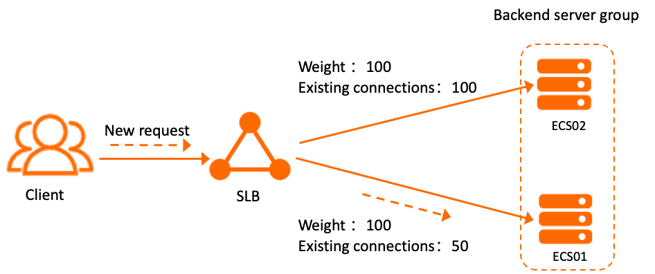
Weighted least connections routes each new request to the backend server with the fewest active connections relative to its weight. If two servers share the same weight, the one with fewer current connections receives the next request. This algorithm works best for consistent connections, such as database connections, where connection count is a meaningful proxy for server load.

For example, with two ECS instances both at weight 100 — one holding 100 active connections and the other holding 50 — new requests go to the instance with 50 connections until the counts balance.

Advantages

1. Real-time load awareness: continuously tracks active connections per server and routes new requests away from busier servers, keeping load balanced under fluctuating traffic.

2. Weight-adjusted fairness: combines connection count with server weight to prevent both overloading high-capacity servers and underutilizing low-capacity ones.

Disadvantages

1. Higher scheduling overhead: compared to round-robin and weighted round-robin, this algorithm must query and compare active connection counts across all backend servers before selecting one, which adds computational cost at scale.

2. Incomplete view of server load: tracks only connections between SLB and the backend server. If the monitoring data is inaccurate or outdated, requests may not be distributed to the server with the least connections. In addition, if the same server belongs to multiple SLB instances, connection counts from a single SLB instance underrepresent the server's true load, which can lead to overloading or underloading.

3. Load spikes when adding new servers: new servers start with zero connections and attract a sudden burst of requests. This can overload them before they warm up, potentially destabilizing the cluster.

When to use

1. Mixed-capacity servers with long-lived connections: combine weights with real-time connection tracking to keep load proportional to each server's capacity, even when connection durations vary widely.

2. Dynamic traffic patterns: when active connections fluctuate significantly over time, the algorithm continuously rebalances traffic without requiring manual weight adjustments.

3. Stability-sensitive workloads: for applications that require consistent response times — such as databases or connection pools — routing new requests to the least-loaded server helps prevent individual servers from becoming bottlenecks.

Consistent hashing

Overview

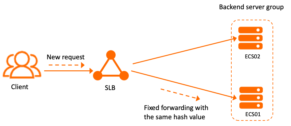
Consistent hashing maps each request to a backend server based on a hash computed from one or more request attributes (hash factors). Requests that share the same hash value always go to the same server — even as the number of backend servers changes. When a server is added or removed, only a minimal subset of requests are rerouted.

Hash factors include:

• Source IP address: requests from the same client IP always reach the same backend server.

• Four elements: hashing uses the combination of source IP address, source port, destination IP address, and destination port. Requests sharing all four values go to the same server.

• QUIC ID: hashing uses the QUIC connection ID, which uniquely identifies each QUIC connection. Hashing based on QUIC IDs can balance loads among connections. Requests with the same QUIC ID are distributed to the same backend server.

• URL query string: requests with the same URL query string are routed to the same backend server.

For example, with two ECS instances in a server group, if the last request was routed to ECS01, any subsequent request with the same hash value is also sent to ECS01.

Advantages

1. Session persistence: requests from the same source are consistently routed to the same backend server, preserving session state without requiring a separate session store. This makes consistent hashing well suited to applications that rely on server-side session data or user-specific cache.

2. Minimal disruption during server changes: when servers are added or removed, only requests whose hash values map to the changed slot are rerouted. The remaining requests continue reaching the same servers as before.

Disadvantages

1. Temporary imbalance after server changes: adding or removing a server causes requests mapped to that server's hash slot to be redistributed. If the number of backend servers increases, fewer requests are rescheduled; if the number decreases, more requests are rescheduled. Until traffic re-equilibrates, some servers may carry a disproportionate share of the load.

2. Increased operational complexity during scale-out: each server change triggers a partial rehash. In environments with frequent scaling events, this ongoing rerouting adds operational overhead and can complicate capacity planning.

When to use

1. Session-persistent applications: use consistent hashing when your application stores session data or user state on individual backend servers and cannot tolerate requests from the same user reaching different servers mid-session.

2. Cache-heavy backends: when backend servers maintain local caches, routing the same requests to the same server maximizes cache hit rates and reduces redundant computation across the cluster.

3. Data locality requirements: in workloads where data partitioned by key must be processed on a specific server — such as sharded databases or stateful stream processing — consistent hashing ensures each key's requests always reach the correct partition.

References

• What is SLB?

• What is ALB?

• What is NLB?

• What is CLB?