Use Grafana to visualize and analyze Nginx logs collected by Simple Log Service (SLS).
-
To quickly try out this feature, you can use the logon-free access link: Demo - Grafana.
-
You can export a dashboard from Simple Log Service (SLS) and import it into Grafana. For more information, see Export a dashboard and import it to Grafana.
Prerequisites
-
Collect Nginx logs. For more information, see Use Nginx configuration mode to collect text logs.
-
Enable and configure indexes. For more information, see Analyze Nginx access logs.
-
Download the data source plugin project package.
Run the following command to download the package:
wget https://github.com/aliyun/aliyun-log-grafana-datasource-plugin/archive/refs/heads/master.zip.NoteThis topic uses the SLS plugin v2.36 as an example.
-
Install Grafana. For more information, see the official Grafana documentation.
Note-
This topic uses Grafana 11.4.0 as an example.
-
If you install Grafana on your local machine, make sure port 3000 is accessible from your browser.
-
To use a pie chart, run the following command to install the Pie Chart plugin.
grafana-cli plugins install grafana-piechart-panel
-
Plugin compatibility
The following table describes the compatibility between Grafana and the SLS plugin.
|
Grafana version |
SLS plugin version |
|
≥8.0.0 |
|
|
<8.0.0 |
Usage notes
If you configure STS-based redirection, the following security conditions must be met:
-
The user associated with the access key of the data source must have the
AliyunRAMReadOnlyAccessandAliyunSTSAssumeRoleAccessaccess policies, permission to call the CreateTicket API, and the required permissions for SLS. -
The RAM role specified in the RoleArn field of the data source must have only the
AliyunLogReadOnlyAccessaccess policy. -
For more information about how this works, see Embed and share console pages.
If you configure logon-free access, verify that the data source is not used in publicly shared Grafana dashboards. Public access can increase traffic costs and expose log content.
For more information about system access policies, see System access policies for Simple Log Service.
Step 1: Install the SLS plugin
-
Run the following command to unzip the plugin package to the Grafana plugin directory.
-
For Grafana installed from a YUM repository or RPM package:
unzip aliyun-log-grafana-datasource-plugin-master.zip -d /var/lib/grafana/plugins -
For Grafana installed from a .tar.gz file:
In this command, {PATH_TO} is the installation path of Grafana.
unzip aliyun-log-grafana-datasource-plugin-master.zip -d {PATH_TO}/grafana-11.4.0/data/plugins
-
-
Modify the Grafana configuration file.
-
Open the configuration file.
-
For Grafana installed from a YUM repository or RPM package: /etc/grafana/grafana.ini
-
For Grafana installed from a .tar.gz file: {PATH_TO}/grafana-11.4.0/conf/defaults.ini
-
-
In the
[plugins]section of the configuration file, set theallow_loading_unsigned_pluginsparameter.allow_loading_unsigned_plugins = aliyun-log-service-datasource
-
-
Restart Grafana.
-
Use the
killcommand to terminate the Grafana process. -
Run one of the following commands to start Grafana.
-
For Grafana installed from a YUM repository or RPM package:
systemctl restart grafana-server -
For Grafana installed from a .tar.gz file:
./bin/grafana-server web
-
-
Step 2: Add a data source
-
Log on to Grafana.
-
In the left-side navigation pane, choose .
-
On the Data Sources tab, click Add data source.
-
On the Add data source page, search for and click log-service-datasource.
-
On the aliyun-log-service-datasource page, configure the following settings.
-
The following table describes the required parameters.
Parameter
Description
Endpoint
The endpoint for the Project, such as
http://cn-qingdao.log.aliyuncs.com. Use your actual endpoint. For more information, see Endpoints.Project
The name of the SLS Project.
AccessKeyID
The AccessKey ID is used to identify a user. For more information, see Access key pair.
We recommend that you grant only the required permissions to a RAM user based on the principle of least privilege. For more information about how to grant permissions to a RAM user, see Create a RAM user and grant permissions and RAM custom policy examples.
AccessKeySecret
The AccessKey secret is used to encrypt and verify a signature string. The AccessKey secret must be kept confidential.
-
The following table describes the optional parameters.
Parameter
Description
Name
The name of the data source. The default value is aliyun-log-service-datasource.
Default
This switch is enabled by default.
Default LogStore
If you omit the Logstore, ensure your access key has the
ListProjectpermission for the current Project.RoleArn
Required for STS-based redirection. Specify the ARN of the RAM role.
HTTP headers
Custom headers are supported and take effect only when the data source type is MetricStore(PromQL). For configuration details, see the
FormValuesettings in Accelerate queries. The following list describes theHeadersfields:-
x-sls-parallel-enable: Specifies whether to enable concurrent computing. Disabled by default. -
x-sls-parallel-time-piece-interval: The time unit for sharding by time range, in seconds. The supported range is[3600, 86400*30]. The default value is21600(6 hours). -
x-sls-parallel-time-piece-count: The number of shards when sharding by time range. The supported range is 1 to 16. The default value is 8. -
x-sls-parallel-count: The global concurrency. The supported range is 2 to 64. The default value is 8. -
x-sls-parallel-count-per-host: The per-host concurrency. The supported range is 1 to 8. The default value is 2. -
x-sls-global-cache-enable: Specifies whether to enable the global cache. Disabled by default.
Region
Supports v4 signature for enhanced security.
-
-
-
After you complete the configuration, click Save & test.
Step 3: Add a dashboard
To add a dashboard to Grafana:
-
In the left-side navigation pane, click Dashboards.
-
On the Dashboards panel, click + Created dashboard. Then, click + Add visualization.
-
On the Select data source page, select aliyun-log-service-datasource as the data source.
-
Add a visualization panel.
The following list describes the settings:
-
Data Source Type: Four types are available, based on syntax (SQL and PromQL) and store type: ALL(SQL), Logstore(SQL), MetricStore(SQL), and MetricStore(PromQL).
-
Logstores support SQL for query and analysis.
-
Metricstores support SQL and PromQL for query and analysis.
-
MetricStore(PromQL) supports adding custom headers on the data source configuration page.
-
-
Logstore list: Select the name of the Logstore to query.
-
Query: Enter a query statement, for example:
* | select count(*) as c, __time__-__time__%60 as t group by t -
ycol:
null -
xcol: Select TimeSeries / Custom and enter
t. -
goto SLS: One-click redirection to the SLS console.
On the Explore and dashboard pages, you can click goto SLS to jump to the SLS console for comparison. You can also use the more powerful features and flexible log search capabilities of the SLS console. When redirected, the query and time information are carried over, eliminating manual entry.
This redirection method takes you directly to the SLS console and requires no configuration. However, you must already be logged in to the SLS console in your browser; otherwise, you will be redirected to the login page.
NoteThis feature is available in the SLS Grafana Plugin version 2.30 and later.
-
-
In the Panel options on the right, enter a Title, and then click Save dashboard in the upper-right corner. In the dialog box that appears, click Save.
Configure template variables
Template variables in Grafana let you dynamically change the data displayed in a chart.
Configure a time interval variable
-
In the upper-right corner of the New dashboard page, click .
-
Click Variables.
-
Click New variable.
-
Configure the template variable with the following parameters and then click Add.
The following table describes the key parameters.
Parameter
Description
Name
The name of the variable, such as myinterval. This variable is used in your configuration and must be entered as
$$myintervalin a query condition.Type
Select Interval.
Label
Set to time interval.
Values
Set to 1m,10m,30m,1h,6h,12h,1d,7d,14d,30d.
Auto Option
Enable the Auto Option switch and keep other parameters at their default settings.
-
Result. After configuration, a time interval drop-down list appears at the top of the dashboard, allowing you to select intervals such as Auto, 1m, 10m, 30m, 1h, 6h, 12h, or 1d.
Configure a domain name variable
-
On the Variables page, click New.
-
Configure the template variable with the following parameters and then click Add.
Parameter
Description
Name
The name of the variable, for example, hostname. This is the variable that you use in your configuration, and if the variable name is hostname, you must specify
$hostnamein the query condition.Type
Select Custom.
Label
Enter a domain name.
Custom Options
If you set the parameter to
*,example.com,example.org,example.net, you can view the access status of all domain names. You can also view the access status ofexample.com,example.org, orexample.netseparately.Selection Options
Keep the default settings.
-
Result. After configuration, a domain name drop-down list appears at the top of the dashboard, allowing you to select * (all domains), example.com, example.org, or example.net.
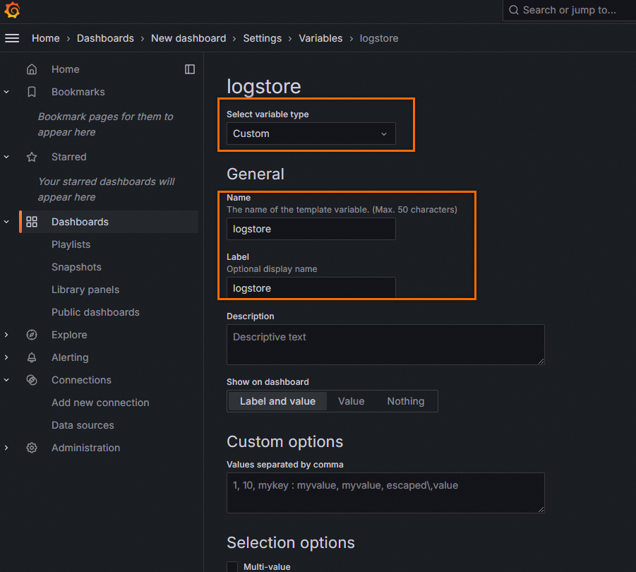
Configure Logstore list variable
-
On the Variables settings page, select the Custom type. The
namefield serves as a unique identifier and must contain the string 'logstore', case-insensitive. In Custom Options, enter the variable values, separated by commas.
-
In the panel editor, change the Logstore list option to your custom variable, select a value, and refresh the dashboard to see the results.
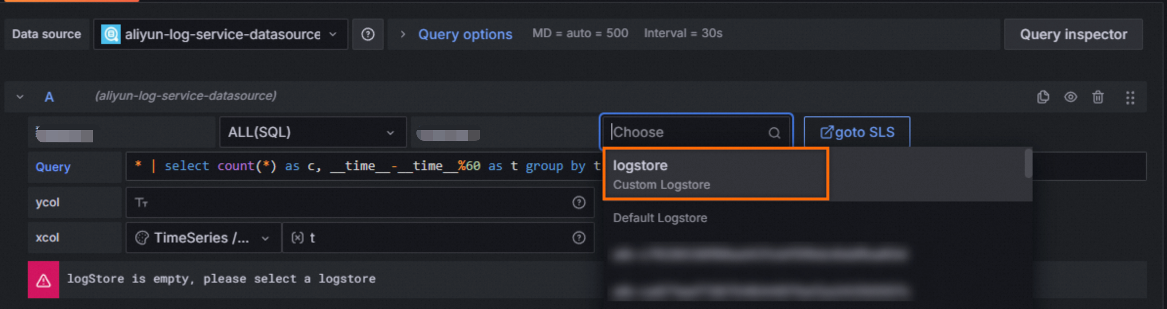


Chart configuration
Stat and Gauge panels
xcol format: stat.
ycol format: <numeric_column>, <numeric_column>.
If you provide a non-numeric column where a numeric column is required, the value is set to 0.
-
Example 1
Panel type: Stat
xcol:
statycol:
PV, deltaPercentquery:
* | select diff[1] as "PV", round((diff[1] - diff[2])/diff[2] * 100, 2) as deltaPercent from (select compare("PV", 86400) as diff from (select count(*) as "PV" from log))The query result is displayed in a Stat panel, showing two numeric metrics: PV and deltaPercent. Positive values are shown in green and negative values are shown in red, with a mini trend line chart below each metric.
-
Example 2
Panel type: Gauge
xcol:
statycol:
cquery:
* | select count(distinct labels['hostname']) as c from (select promql_query('${metricName}{cluster =~ "${cluster}"}') from metrics ) limit 100000The query result is displayed in a Gauge panel. The value is shown as an arc indicator on a gauge, with the arc transitioning from green to red to represent the value range.
Pie chart
xcol format: pie.
ycol format: <grouping_column>, <numeric_column>.
-
Example 1
Panel type: Pie Chart
xcol:
pieycol:
request_method, cquery:
request_method: "$method" | select count(*) as c, request_method group by request_methodThe query result is displayed as a pie chart showing the distribution of various HTTP request methods, such as GET, POST, PUT, and DELETE.
-
Example 2
Panel type: Pie Chart
xcol:
pieycol:
http_user_agent, pvquery:
* | select count(1) as pv, case when http_user_agent like '%Chrome%' then 'Chrome' when http_user_agent like '%Firefox%' then 'Firefox' when http_user_agent like '%Safari%' then 'Safari' else 'unKnown' end as http_user_agent group by case when http_user_agent like '%Chrome%' then 'Chrome' when http_user_agent like '%Firefox%' then 'Firefox' when http_user_agent like '%Safari%' then 'Safari' else 'unKnown' end order by pv desc limit 10The query result is displayed as a pie chart showing the percentage of traffic from different browsers: Chrome, Firefox, Safari, and unKnown.
-
Other use cases
The format for Stat panels can also be applied to pie charts to produce a valid visualization.
Panel type: Pie Chart
xcol:
statycol:
hostNameNum, ipNumquery:
* | select count(distinct labels['hostname']) as hostNameNum, count(distinct labels['ip']) + 20 as ipNum from (select promql_query('${metricName}{cluster =~ ".*"}') from metrics ) limit 100000The query result is displayed as a pie chart showing the proportion of the hostNameNum and ipNum metrics.
Time series
xcol format: <time_column>.
ycol format: <numeric_column> [, <numeric_column>, ...] (Logstore syntax) or <labels / grouping_column>#:#<numeric_column> (Metricstore syntax or log aggregation syntax).
-
Example 1
Panel type: Time series
xcol:
timeycol:
pv, uvquery:
* | select __time__ - __time__ % $${myinterval} as time, COUNT(*)/ 100 as pv, approx_distinct(remote_addr)/ 60 as uv GROUP BY time order by time limit 2000The query result is displayed as a time series line chart showing the trends of two series, pv and uv, over time.
-
Example 2
Panel type: Time series
xcol:
timeycol:
labels#:#valuequery:
* | select time, * from (select promql_query_range('${metricName}') from metrics) limit 1000The query result is displayed as a time series line chart, where each series is automatically named and grouped by its labels.
-
Example 3
You can also use SQL to customize the display of time series labels.
Panel type: Time series
xcol:
timeycol:
customLabelsExtract#:#valuequery:
* | select concat(labels['ip'], ' -> ', labels['cluster']) as customLabelsExtract, value from (select promql_query_range('${metricName}') from metrics) limit 1000The query result is displayed as a time series line chart, with series names defined by the custom SQL field customLabelsExtract (format:
IP -> cluster).
Bar chart
xcol format: bar.
ycol format: <grouping_column>, <numeric_column> [, <numeric_column>, ...].
-
Example 1
Panel type: Bar chart
xcol:
barycol:
host, pv, pv2, uvquery:
* | select host, COUNT(*)+10 as pv, COUNT(*)+20 as pv2, approx_distinct(remote_addr) as uv GROUP BY host ORDER BY uv desc LIMIT 5The query result is displayed as a horizontal bar chart comparing the pv, pv2, and uv metrics for each host.
Table
The Table panel supports sorting by time with nanosecond precision if a nanosecond field exists.
Supports modifying the totalLogs count. The default is 100, the minimum is 1, and the maximum is 5000. This applies only to query statements, not analysis statements.
xcol syntax: <empty>.
ycol format: Leave this field empty or specify <display_column> [, <display_column>, ...].
-
Example 1
Panel type: Table
xcol:
Table/Logycol:
<empty>query:
* | select __time__ - __time__ % 60 as time, COUNT(*)/ 100 as pv, approx_distinct(remote_addr)/ 60 as uv GROUP BY time order by time limit 2000The query result is displayed in a table with columns for time, pv, and uv.
Logs
xcol syntax: <empty>.
ycol syntax: <empty>.
Example
Panel type: Logs
xcol: <Empty>
ycol: <Empty>
query:
host: www.vt.mock.comThe query result is displayed in a Logs panel showing raw log entries, with each entry displaying key-value pairs for its fields.
Traces
Panel type: Traces
xcol: trace
ycol: <empty>
query:
traceID: "f88271003ab7d29ffee1eb8b68c58237"The query result is displayed in a Traces panel showing the trace information. The left side lists the Service & Operation, and the right side shows a Gantt chart timeline for each span, illustrating the hierarchy and duration of the trace.
This example uses a Logstore that contains trace data. You must enable the Trace service in SLS. SLS supports native ingestion of OpenTelemetry trace data and also supports ingesting trace data from other tracing systems. For more information, see Overview of ingesting trace data.
In Grafana 10.0 and later, span filtering for trace data is supported. If you are using an older version of Grafana, you can also define custom span filters in your query. For example:
traceID: "f88271003ab7d29ffee1eb8b68c58237" and resource.deployment.environment : "dev" and service : "web_request" and duration > 10GeoMap
xcol format: map.
ycol format: <country_column>, <geolocation_column>, <numeric_column>.
Example
Panel type: GeoMap
xcol: map
ycol: country, geo, pv
query:
* | select count(1) as pv ,geohash(ip_to_geo(arbitrary(remote_addr))) as geo,ip_to_country(remote_addr) as country from log group by country having geo <>'' limit 1000The query result is displayed on a GeoMap, showing the distribution of traffic across different regions on a world map. The size of the circles indicates the volume of traffic.
FAQ
-
Where are Grafana logs stored?
Grafana logs are stored in the following directories:
-
macOS: /usr/local/var/log/grafana
-
Linux: /var/log/grafana
-
-
What should I do if aliyun-log-plugin_linux_amd64: permission denied appears in the logs?
Grant execution permissions to the dist/aliyun-log-plugin_linux_amd64 directory in the plugin directory.