To optimize a model with TensorRT, you compile a model trained using a framework like PyTorch or TensorFlow into the TensorRT format, then execute it with the TensorRT inference engine. This process accelerates model execution on NVIDIA GPUs, making it ideal for applications that require high real-time performance. This article explains the model training and compilation process and offers best practices for optimizing model inference performance with TensorRT.
Before you begin
To better understand how to optimize model inference performance with TensorRT:
-
Review the Introduction to TensorRT and the TensorRT Cookbook source code to understand the basics of TensorRT's architecture and usage.
-
Verify that your CUDA version is compatible with TensorRT. As TensorRT is designed for NVIDIA GPUs, it requires NVIDIA hardware. For more information, see the official TensorRT documentation.
-
This article uses Nsight Systems to profile system-wide activity, including kernel read/write operations, scheduling between kernels, SM occupancy, and asynchronous execution between the CPU and GPU.
Actual performance gains depend on the model's type and size, and the specific graphics card.
Model compilation example
-
This example demonstrates a simple training workflow using an existing ResNet-18 model. You can follow this example to learn the concepts and techniques for model performance analysis and optimization.
-
TensorRT version: v8.6.1. For other versions, see the TensorRT Download page.
-
PyTorch version: 2.2.0.
-
GPU: V100-SXM2-32GB. This tutorial uses the official NVIDIA PyTorch image.
Pull the official NVIDIA PyTorch Docker image:
docker pull nvcr.io/nvidia/pytorch:24.01-py3. Note: When starting the Docker container, mount shared memory (docker run --shm-size=) and share the host machine's IPC namespace (--ipc=host).
-
-
Train the model and generate an ONNX model file.
The following code pulls a pre-trained ResNet-18 model, performs simple training, and saves the model in ONNX format.
-
Save the TensorRT compilation script.
The following script compiles the model. Save it as
0_build.py. -
Save the baseline model script.
Save the following baseline model script as
1_baseline.py. -
Run inference optimization and view the process.
After completing the setup, run the following shell commands.
python 0_build.py
mkdir -pv reports
nsys profile -w true \
	-t cuda,nvtx,osrt,cudnn,cublas \
	--cuda-memory-usage=true \
	--cudabacktrace=all \
	--cuda-graph-trace=node \
	--gpu-metrics-device=all \
	-f true \
	-o reports/1_baseline \
	python 1_baseline.py
When the run completes, it generates a
1_baseline.nsys-repfile in the ./reports directory. Import this file intoNsight Systemsto view the timeline, as shown below.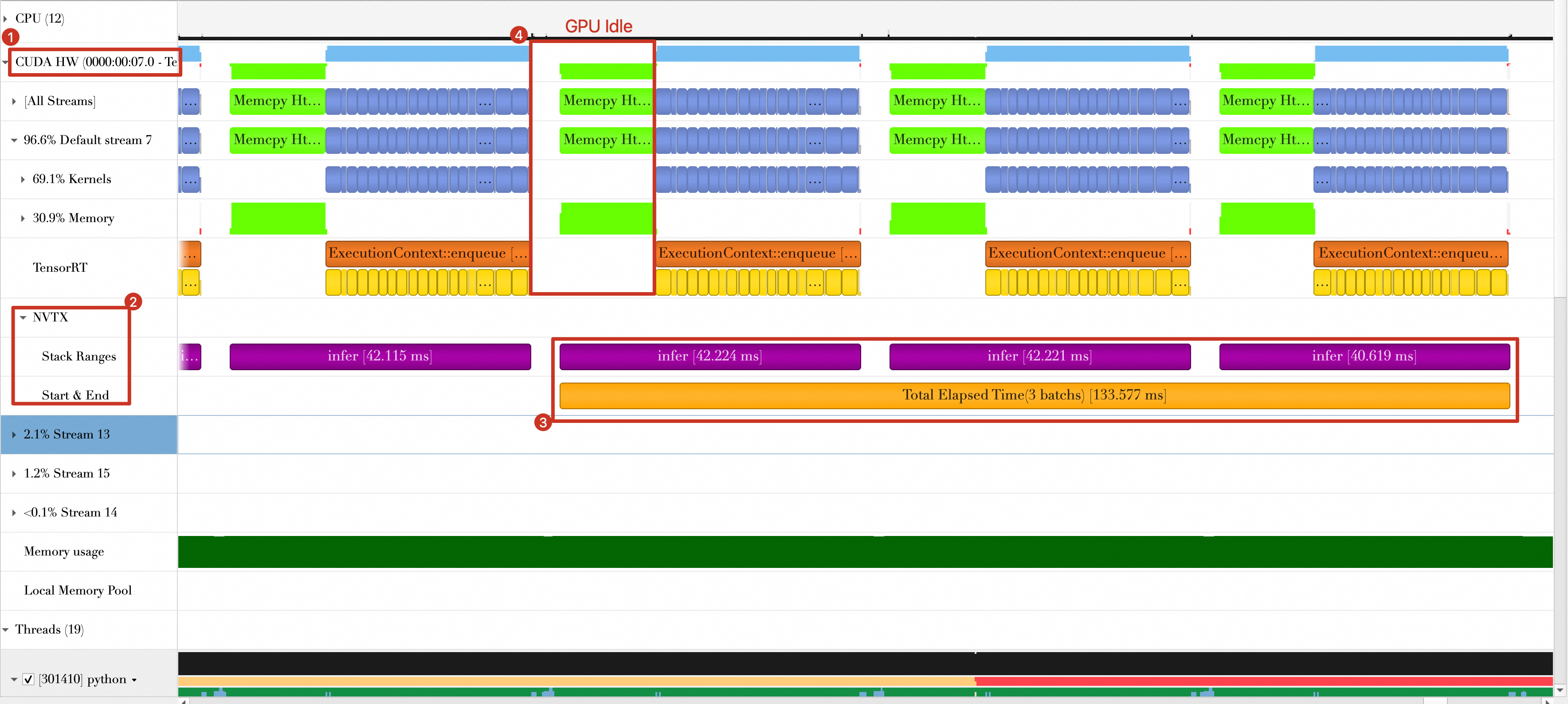
The timeline shows the following:
-
The total time for the last three batches is approximately 133.577 ms.
-
Between batches, the GPU is briefly idle (labeled 4 in the figure), caused by batch data transfer and the printing of results on the host.
-
Model optimization
Approach 1: Reuse allocated GPU memory
-
Problem analysis.
In the baseline code, GPU memory is allocated for each batch and then deallocated after the batch is processed. Frequent memory allocation and deallocation is time-consuming and can create a performance bottleneck.
-
Solution design.
Reusing allocated GPU memory can reduce batch processing time. Modify the baseline code to allocate GPU memory when processing the first batch, and then reuse it for subsequent batches.
The complete code is shown below. Note: Only the
inferandinfer_oncefunctions have been modified; the rest of the code is identical to the baseline. Save the code as2_reuse_buffers.py. -
Run the following shell command to profile the script.
nsys profile -w true \ -t cuda,nvtx,osrt,cudnn,cublas \ --cuda-memory-usage=true \ --cudabacktrace=all \ --cuda-graph-trace=node \ --gpu-metrics-device=all \ -f true \ -o reports/2_reuse-buffers \ python 2_reuse-buffers.py -
Running the command creates the file
2_reuse-buffers.nsys-repin the./reportsdirectory. Import this file intoNsight Systems. As shown in the timeline below,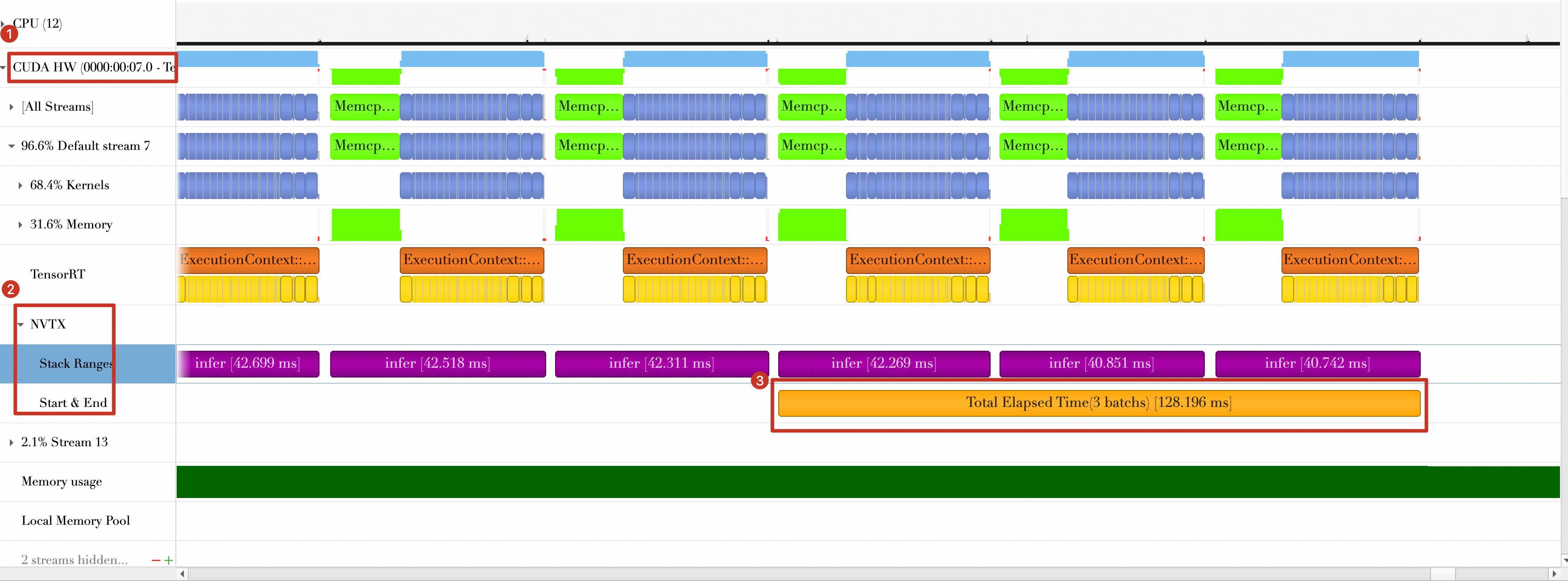 the total time for the last three batches is approximately 128.196 ms, which is a 5.381 ms reduction from the baseline (133.577 ms - 128.196 ms).
Approach 2: Use pinned memory
-
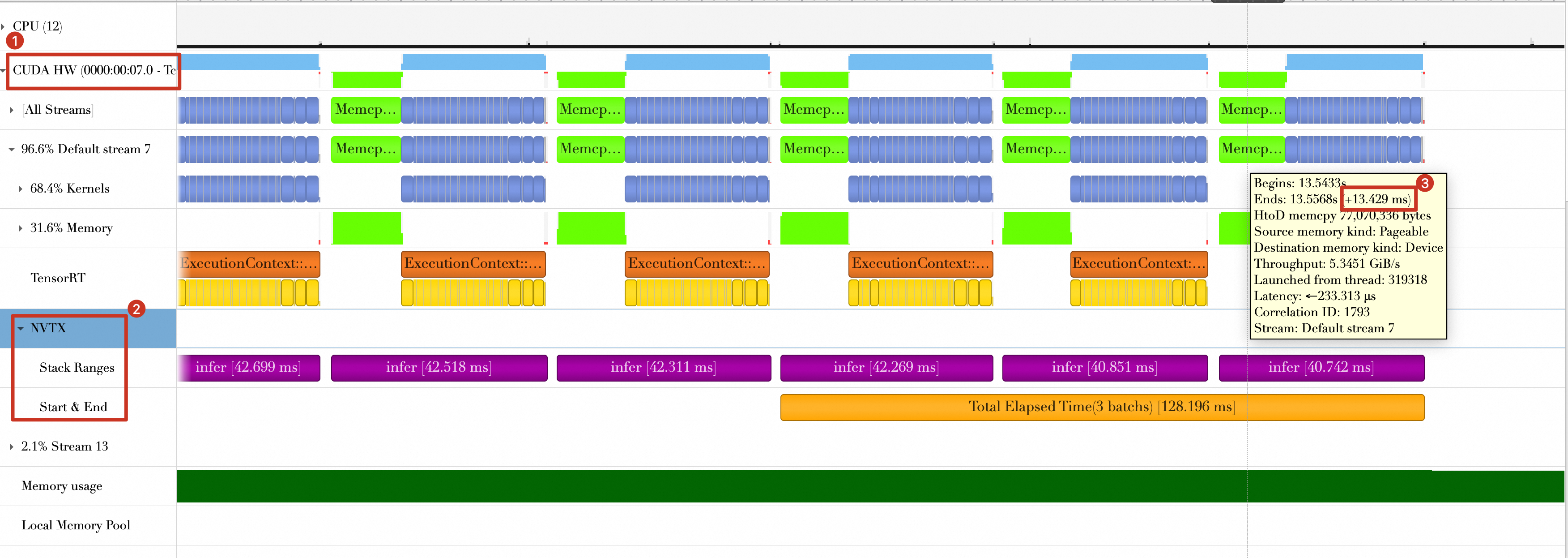
Problem analysis
Building on Approach 1, we continue to look for optimization opportunities. The timeline from the previous step shows that during the host-to-device data transfer, which takes approximately 13 ms, the GPU is idle. Shortening this data transfer time is therefore key to reducing the overall batch processing time.
-
Solution design
To accelerate data transfers, we will use pinned memory. When generating random data, store it in pinned memory using the
data_generation_with_pin_memoryfunction. This requires some modifications to themainfunction, but the rest of the code remains largely unchanged. The code is saved in3_use-pin-memory.py. -
Run the following shell command.
nsys profile -w true \ -t cuda,nvtx,osrt,cudnn,cublas \ --cuda-memory-usage=true \ --cudabacktrace=all \ --cuda-graph-trace=node \ --gpu-metrics-device=all \ -f true \ -o reports/3_use-pin-memory \ python 3_use-pin-memory.py -
After the command finishes running, it generates a
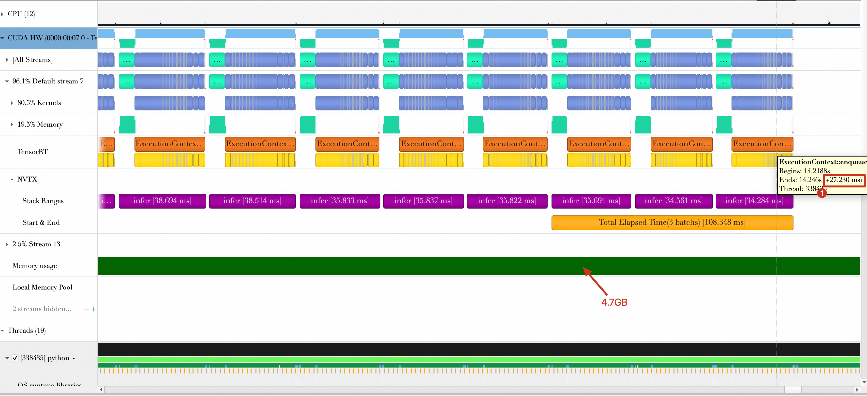
3_use-pin-memory.nsys-repfile in the ./reports directory. Import this file intoNsight Systems. The timeline is shown below.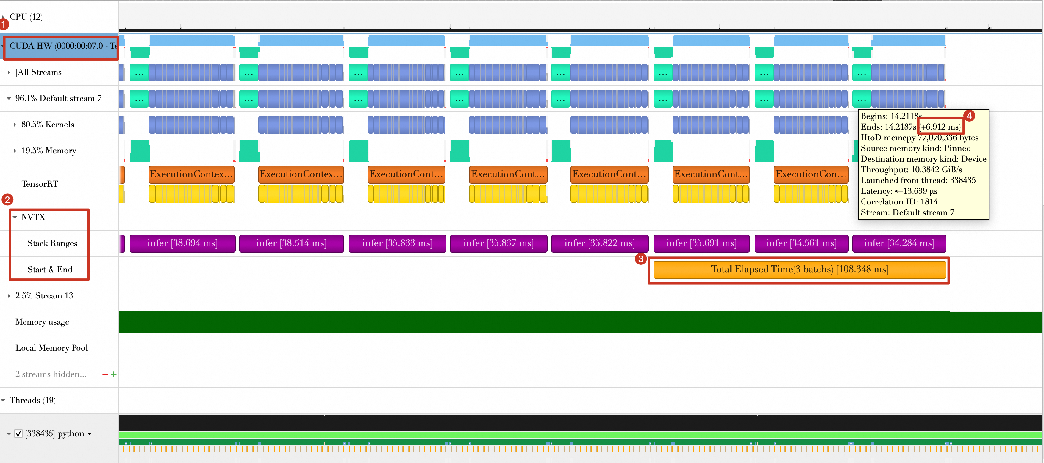 The figure shows the following:
-
The total time for the last three batches is now approximately 108.348 ms, a reduction of 19.848 ms (down from 128.196 ms).
-
The batch transfer time is reduced from 13.429 ms to 6.912 ms.
-
Approach 3: Use FP16 (or INT8) precision
-
Problem analysis
The timeline from Approach 2 shows a computation time of approximately 27.230 ms per batch and memory consumption of 4.7 GB.
-
Solution design
You can reduce batch computation time by enabling a lower precision, such as FP16 or INT8, when you compile the model. To enable FP16, add the following line to the
BuilderConfig.config.set_flag(trt.BuilderFlag.FP16) -
The
0_build.pyscript includes an--fp16option to enable FP16 mode during compilation. Copy3_use-pin-memory.pyto4_use-fp16.pyand run the following shell script.python 0_build.py --fp16 # Enable FP16 mode nsys profile -w true \ -t cuda,nvtx,osrt,cudnn,cublas \ --cuda-memory-usage=true \ --cudabacktrace=all \ --cuda-graph-trace=node \ --gpu-metrics-device=all \ -f true \ -o reports/4_use-fp16 \ python 4_use-fp16.py -
After the run completes, a file named
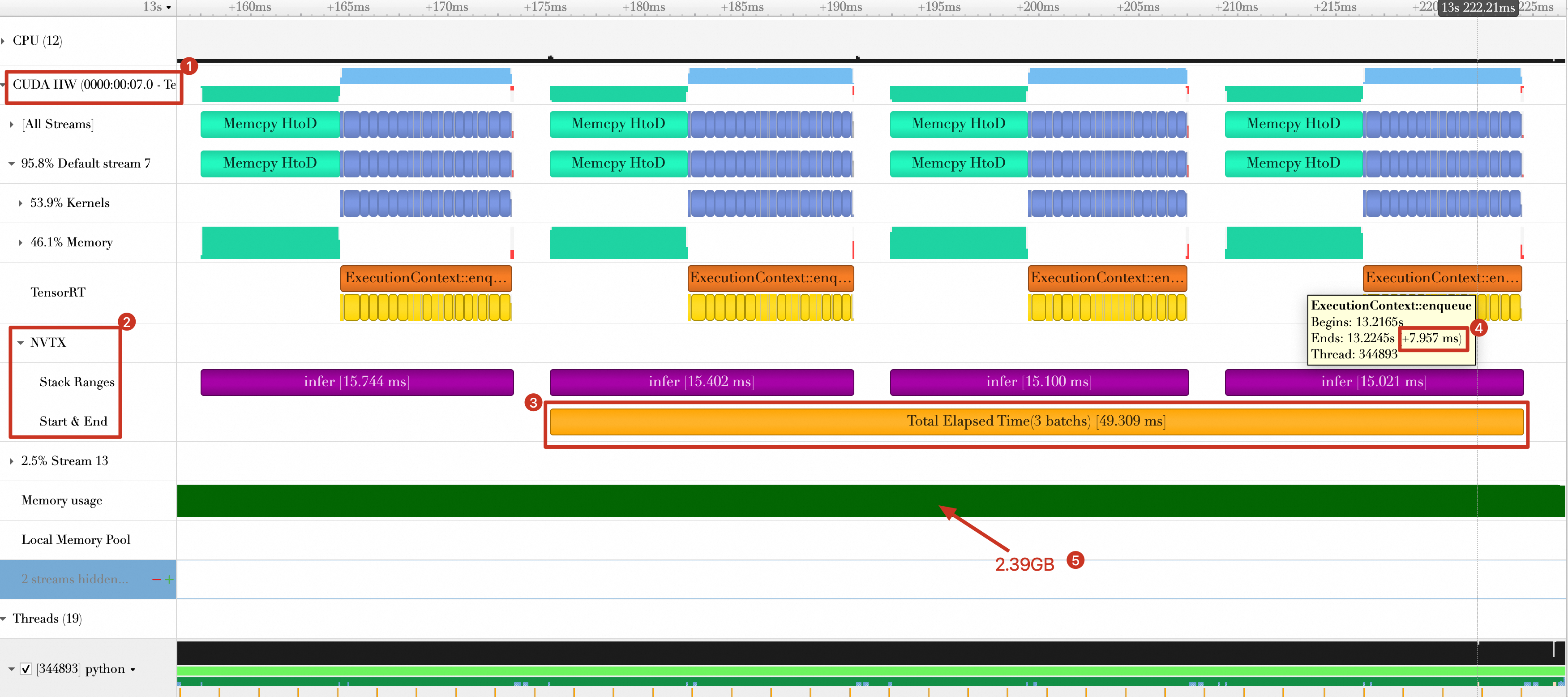
4_use-fp16.nsys-repis generated in the./reportsdirectory. Import this file intoNsight Systemsto view the timeline. The results are as follows:
-
The total processing time for the three batches is reduced from 108.348 ms to 49.309 ms.
-
The per-batch computation time is reduced from 27.230 ms to 7.957 ms.
-
GPU memory usage is reduced from 4.7 GB to 2.39 GB.
ImportantIn production, you must also run a calibration process to ensure the accuracy of the quantized model. For more information, see the official TensorRT documentation.
-
 The results are as follows:
Approach 4: Overlapping data transfer and data computation
-
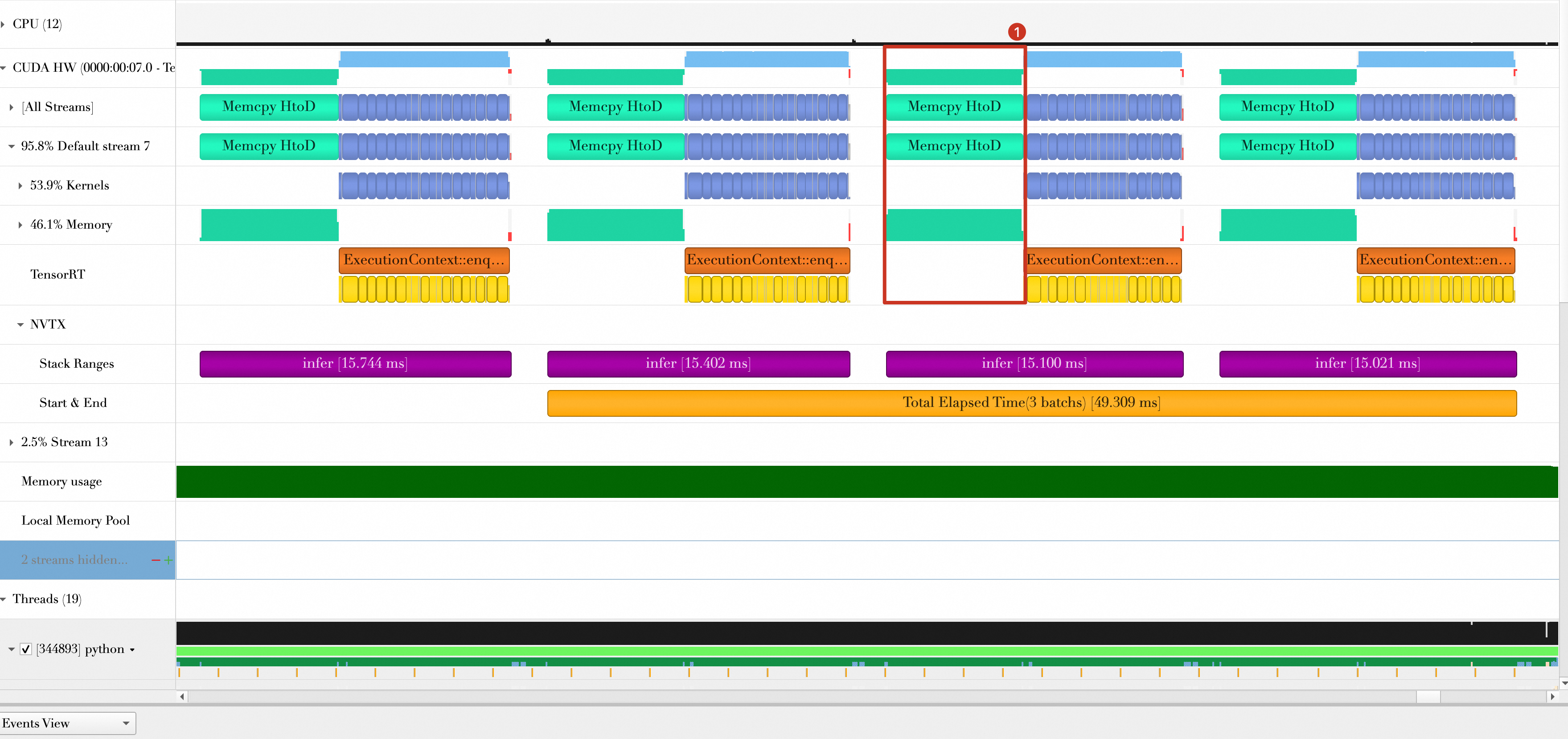
Problem analysis
After quantization, data transfer time becomes significant relative to computation time. Consequently, simply reducing transfer time is no longer a sufficient optimization.
-
Solution design
Achieving overlapping data transfer and data computation requires using CUDA streams.
Modify the code as follows:
-
Create two CUDA streams: one to transfer data from the host to the device, and another for computation and returning results.
-
Create three CUDA events for synchronization between the CUDA streams, and between the GPU and the host.
-
Pre-transfer the data for the first batch. Then, while the GPU computes the first batch, transfer the data for the second batch. This pipelined approach continues for subsequent batches.
Save the following code as 5_multi-streams.py.
-
-
Run the following shell command.
python 0_build.py --fp16 nsys profile -w true \ -t cuda,nvtx,osrt,cudnn,cublas \ --cuda-memory-usage=true \ --cudabacktrace=all \ --cuda-graph-trace=node \ --gpu-metrics-device=all \ -f true \ -o reports/5_multi-streams \ python 5_multi-streams.py -
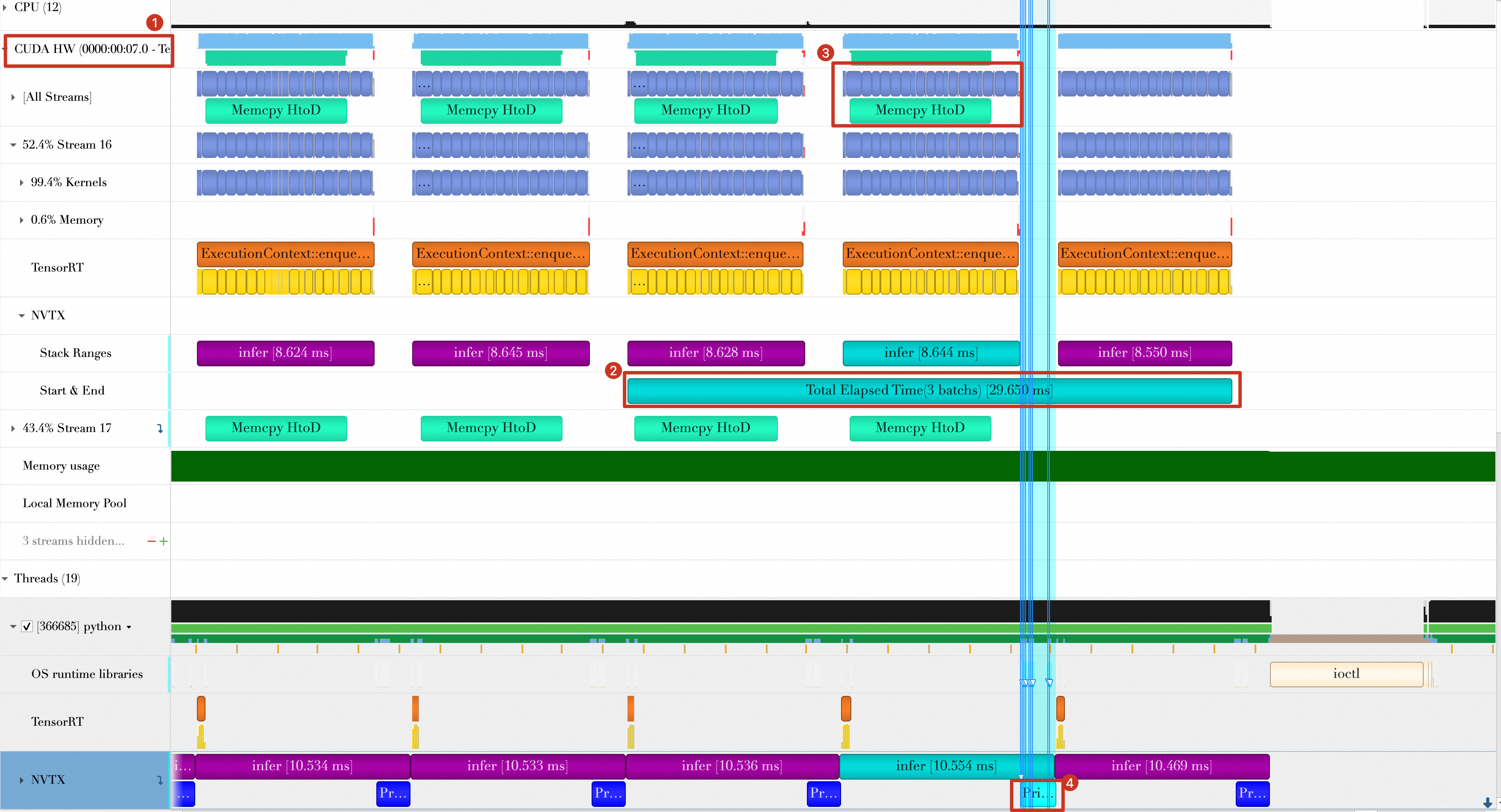
The results are shown in the timeline below.
The timeline shows the following:
-
The total time for three batches is reduced from 49.309 ms to 29.650 ms.
-
In the timeline for Approach 3, data transfer (from the host to the device, labeled
Memcpy HtoD) and computation (the blue sections) run serially. This optimization enables them to run in parallel, as indicated by label 3. -
A noticeable gap remains between batches, which the timeline reveals is caused by the
print_resultfunction.
-
Approach 5: Multi-threading for output processing
-
Problem analysis
In the timeline for Approach 4, there are still gaps between batches. These gaps are caused by the
print_resultfunction, which leaves the GPU idle while printing the output. -
Solution design
You can use Python multi-threading to offload output processing to a separate thread, freeing the main thread to continue execution.
Modify the
inferfunction to create a thread that executes theprint_resultfunction. The complete code is shown below, saved in6_multi-threads.py. -
Run the following shell commands.
python 0_build.py --fp16 nsys profile -w true \ -t cuda,nvtx,osrt,cudnn,cublas \ --cuda-memory-usage=true \ --cudabacktrace=all \ --cuda-graph-trace=node \ --gpu-metrics-device=all \ -f true \ -o reports/6_multi-threads \ python 6_multi-threads.py -
The timeline shows that the
print_resultfunction now overlaps with GPU computation and data transfer instead of executing serially. After running6_multi-threads.py, the Nsight Systems timeline shows that in the GPU hardware row, Stream 16 (kernel computation) and Stream 17 (HtoD memory copy) run in parallel, with 52.4% and 43.5% utilization, respectively. The Threads area shows multiple Python threads working simultaneously, and the NVTX row shows multiple Print Result markers. This confirms that output processing completes asynchronously in a separate thread and no longer blocks the main inference pipeline. As a result, the total time for the last three batches decreases by 2.86 ms, from 29.650 ms to 26.787 ms. Performance analysis of6_multi-threads.pyin Nsight Systems shows that each TensorRT ExecutionContext::enqueue call takes about 8.5–8.7 ms, the NVTX infer range takes about 8.6–8.75 ms, and the NVTX Total Elapsed Time(3 batchs) ranges are 26.787 ms and 27.173 ms. The parallel execution of the compute and copy streams, visible at the CUDA HW level, validates that this multi-threading approach is effective.
Approach 6: Using CUDA Graph
-
Problem analysis.
In the timeline for Approach 5, each batch computation involves 25 separate kernel launches, each incurring overhead. A performance analysis of the TensorRT inference task in Nsight Systems on a Tesla V100-SXM2-32GB GPU shows that a single inference takes about 9.107 ms, while three batches take a total of 27.173 ms. Searching for the
launchkeyword reveals 25 kernel launches. For one of these kernels,volta_first_layer_filter7x7_fwd_execute_flt_k_64_kernel_trt, the actual execution time is only 6.576 μs, but its launch latency is as high as 133.405 μs. This indicates that the launch overhead for many small kernels far exceeds their execution time, making this workload an ideal candidate for optimization with CUDA Graph. -
Solution design.
CUDA Graph, a feature introduced in CUDA 10.0, allows developers to capture a series of CUDA operations, such as memory transfers and kernel executions, and organize them into a directed acyclic graph. This graph acts as a snapshot of a sequence of operations on CUDA streams. Once captured, the graph can be replayed multiple times with minimal CPU overhead, which reduces CPU-GPU interaction and improves overall efficiency. You can use CUDA Graph to capture the operations a TensorRT engine requires for inference, including memory copies and kernel executions. This reduces CPU scheduling overhead, which can significantly improve performance, especially for repetitive inference tasks.
ImportantUsing CUDA Graph can be complex. It typically requires a solid understanding of CUDA programming and how to configure and execute inference in TensorRT. Furthermore, the effectiveness of CUDA Graph depends on the use case, as not all CUDA operations support graph capture. The model in this article is an example of a workload that cannot use CUDA Graph because it contains unsupported operations.
The following example shows how to use CUDA Graph in TensorRT by modifying the
infer_oncefunction. -
After running the code, the following error occurs. This likely means the model contains CUDA operations that do not support graph capture.
[03/04/2024-12:34:39] [TRT] [E] 1: [caskUtils.cpp::createCaskHardwareInfo::852] Error Code 1: Cuda Runtime (operation not permitted when stream is capturing)
cudaError_t.cudaErrorStreamCaptureInvalidated
cudaError_t.cudaErrorInvalidValue
For a CUDA Graph example, see CUDA Graph.
Approach 7: Multiple CPU threads and contexts
-
Problem Analysis
Previous approaches processed data using a single execution context. A single context cannot process multiple batches in parallel because each context maintains intermediate caches for inference, and these caches can only serve one batch at a time.
-
Solution Design
Multiple CPU threads on the host can submit batch processing requests for TensorRT to process in parallel. TensorRT supports this by allowing the creation of multiple, independent contexts.
The following example creates two contexts that use the same optimization profile. This requires enabling the shared profile option when building the engine. The 10 generated batches are split into two groups of five, and each context processes one group.
The complete code is shown below, saved as
8_multi_cpu_threads.py. -
The preceding code starts two Python threads. Each thread processes five batches, creates its own context, and runs inference independently. Then, execute the following shell script.
python 0_build.py --fp16 --share-profile # Enable profile sharing nsys profile -w true \ -t cuda,nvtx,osrt,cudnn,cublas \ --cuda-memory-usage=true \ --cudabacktrace=all \ --cuda-graph-trace=node \ --gpu-metrics-device=all \ -f true \ -o reports/8_multi-context \ python 8_multi-context.py -
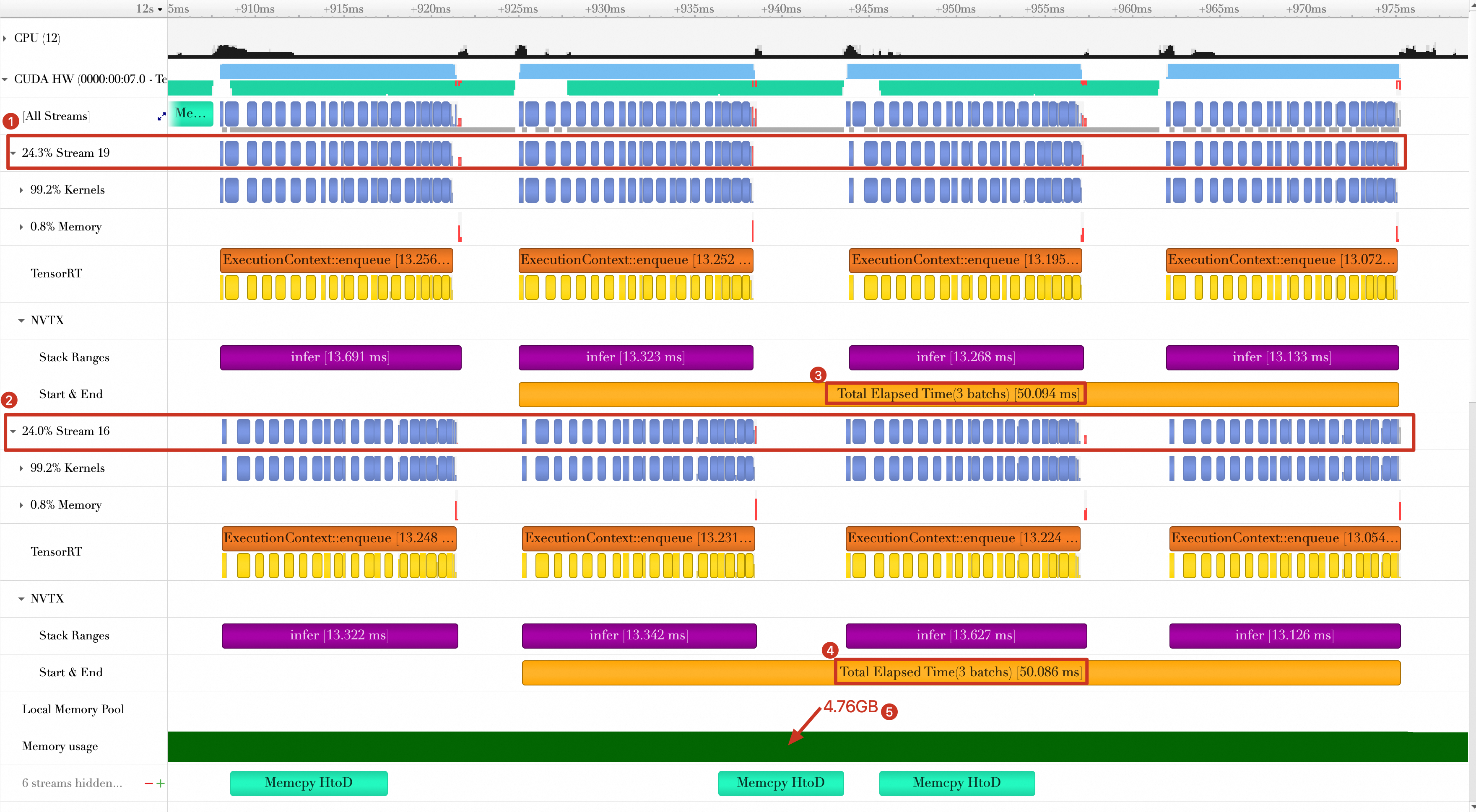
The timeline shows the following results.
-
GPU compute runs in parallel across two streams (Stream 19 and Stream 16).
-
On each stream, processing the last three batches takes about 50 ms. Since two streams run in parallel, the effective processing time for these three batches is approximately 25 ms (50 ms / 2), yielding an average of about 8.3 ms per batch. This parallel execution leads to fuller GPU utilization, but the increased contention on each stream also highlights the risk of computational overload.
-
GPU memory usage is approximately double that of a single-context inference run.
-
Approach 8: Multiple profiles with Dynamic Shape
-
Problem analysis
The Dynamic Shape feature improves kernel flexibility by allowing a model to process input data of various sizes. However, in practice, you might need to compile multiple versions of a kernel to optimally handle different input sizes or other conditions. This is where multiple profiles become useful. You can implement multiple profiles by adding several compilation options when you build the engine. For example, you can use different thread block sizes or other optimization parameters for different input sizes. In some scenarios, the performance of Dynamic Shape can degrade significantly when the min-opt-max range is too wide.
-
Solution design
The solution is to use multiple optimization profiles, each corresponding to a narrower min-opt-max range.
To demonstrate how to use multiple profiles, the following code simplifies and modifies the baseline example.
First, modify the
0_build.pyscript. During the build phase, you need to create two optimization profiles and set themin-opt-maxshape for each. This code is saved in9_multi-profiles-build.py. -
Next, prepare the inference script and save it as
9_multi-profiles.py. The script prepares two datasets,data0anddata1, with shapes of[16,3,224,224]and[128,3,224,224], respectively. Without multiple profiles, you would need to allocate new GPU memory each time the data shape changes. -
After the setup is complete, run the following shell script.
python 9_multi-profiles-build.py --output resnet18-multi-profiles.plan nsys profile -w true \ -t cuda,nvtx,osrt,cudnn,cublas \ --cuda-memory-usage=true \ --cudabacktrace=all \ --cuda-graph-trace=node \ --gpu-metrics-device=all \ -f true \ -o reports/9_multi-profiles \ python 9_multi-profiles.py -
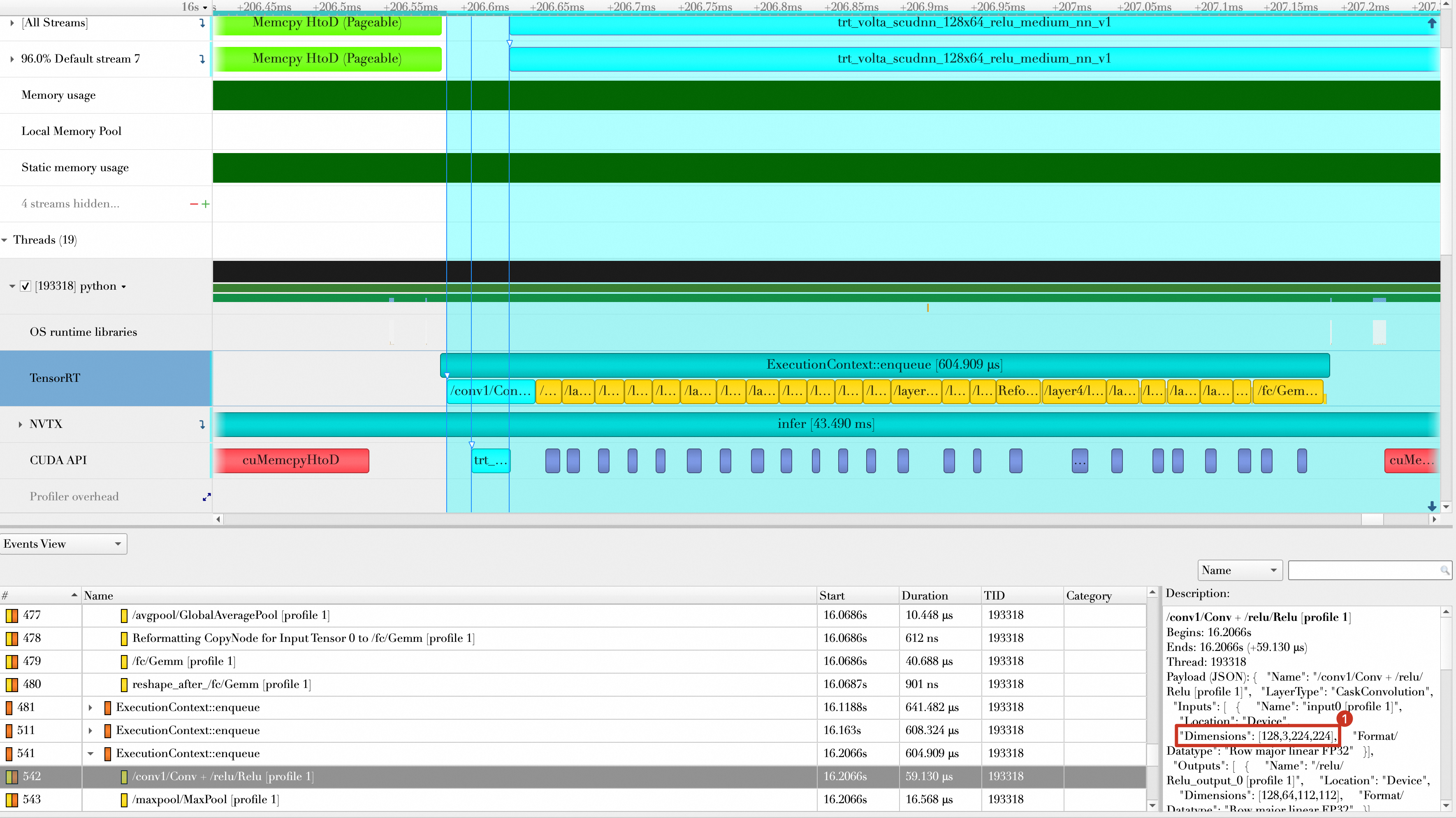
Import the results into
Nsight Systems. The result is shown below. In the Nsight Systems performance analysis, select the/conv1/Conv+/relu/Relulayer. The Description panel on the right shows that its input dimension is[16,3,224,224], which confirms that the inference for the first 10 batches used the shape configuration from the first optimization profile.The shape for the next 10 batches is
[128,3,224,224].For more information about Dynamic Shape, see the TensorRT Cookbook.
Summary
These optimization techniques reduced the processing time for three batches from 133.577 ms to about 25 ms. For more on TensorRT's advanced features and optimization techniques, see the TensorRT Cookbook.