In deep learning, you can use Nsight Systems and Nsight Compute to analyze and optimize the performance of AI applications. This topic demonstrates how to use Nsight Systems for this purpose.
AI performance analysis and optimization procedure
NVIDIA provides profiling tools for CUDA-level analysis. The most important tools in the Nsight family are Nsight Systems, Nsight Compute, and Nsight Graphics.
In deep learning, you can use Nsight Systems and Nsight Compute for performance analysis and optimization. Nsight Graphics is rarely used.

During the performance optimization cycle, first use Nsight Systems to obtain a global view of the application. Then, use Nsight Compute to investigate specific issues in-depth. After optimization, use Nsight Systems again to re-evaluate the overall effect. Repeat this process until you achieve the desired performance level.
For example, you can follow this procedure to analyze and optimize AI application performance using Nsight Systems and Nsight Compute:
Use Nsight Systems to observe the exact runtime of a CUDA kernel and analyze the program.
If a kernel runs too long, use Nsight Compute to further analyze and optimize that CUDA kernel.
After optimizing the CUDA kernel, use Nsight Systems to profile the program again. Repeat this step until the program's performance meets your expectations.
Benefits and limitations of Nsight Systems
Benefits
Cross-platform visualization:
Nsight Systems captures and visualizes system-wide activity in real time, including CPU, GPU, network interface controller (NIC), storage, and other accelerator execution and resource usage. This helps developers better understand interactions and dependencies between hardware components.
Deep hardware insights:
Nsight Systems provides device-level profiling metrics to reveal GPU workload details. For example:
It shows GPU utilization to identify idle periods or overloads.
It analyzes kernel scheduling and execution, including whether grid dimensions are set appropriately and whether stream concurrency fully uses GPU resources.
It checks the occupancy of each streaming multiprocessor (SM) and warp scheduling efficiency.
It confirms whether the application effectively uses hardware units such as Tensor Cores, which are designed specifically for machine learning and deep learning tasks.
It calculates the GPU instruction execution rate to assess performance bottlenecks and potential optimization opportunities.
Automatic optimization suggestions:
Nsight Systems provides Expert Systems Analysis. If the tool detects potential optimization points in your program, it offers optimization suggestions.
Limitations
Modified launch commands affect program performance:
Profiling requires you to launch the target application through its command line interface (CLI), such as
nsys profile. This operation may increase the startup time or alter the process environment, which can affect the original application's performance.
Lacks continuous profiling capability:
For long-running applications, especially those with intermittent GPU usage such as online inference services, Nsight Systems may collect massive amounts of data, which makes the results hard to read and analyze.
Environment preparation
This example uses a V100-SXM2-32GB GPU and NVIDIA's official PyTorch Docker image (nvcr.io/nvidia/pytorch:24.03-py3) to run code.
NVIDIA's official PyTorch image comes pre-installed with Nsight Systems, so no additional installation is needed.
Create a cluster with GPU nodes and enable GPU monitoring. For more information, see Add GPU nodes to a cluster and Enable GPU monitoring for a cluster.
For more information about the GPU-accelerated instance families supported by ACK clusters, see GPU-accelerated instance families supported by ACK.
Set up the PyTorch environment.
Use Arena to set up the PyTorch environment
Install the latest version of Arena. For more information, see Configure the Arena client.
Run the following command to modify the values.yaml file.
vi ~/charts/pytorchjob/values.yamlOpen the file and change the values of the
shmSizeandprivilegedparameters as follows:shmSize: 20Gi # Use the shmSize parameter to specify shared memory size. privileged: true # To use pytorch Profiler, run the container in privileged mode (privileged=true).Run the following command to set up the PyTorch environment.
You can use Arena to submit a simple PyTorch job request to the ACK cluster. The job does not perform actual deep learning training. Instead, it runs the
sleep 10dcommand to simulate a continuously running process for testing and verifying the job submission workflow.arena submit pytorch \ --name=workspace \ --gpus=1 \ --image=nvcr.io/nvidia/pytorch:24.03-py3 \ "sleep 10d"Expected output:
pytorchjob.kubeflow.org/workspace created
INFO[0005] The Job workspace has been submitted successfully
INFO[0005] You can run `arena get workspace --type pytorchjob -n default` to check the job status
The output shows that the PyTorch job was created successfully.
Run the following command to check if the job is in the
Runningstate.arena get workspaceAfter the job enters the
Runningstate, run the following command to enter the PyTorch container for profiling.arena attach workspaceExpected output:
Hello! Arena attach the container pytorch of instance workspace-master-0Check if Nsight Systems is installed in the PyTorch container.
nsys profile --help
Use kubectl to set up the PyTorch environment
Copy and paste the following content into the pytorch-workspace.yaml file to create a Deployment.
apiVersion: apps/v1
kind: Deployment
metadata:
  name: pytorch-workspace
spec:
  selector:
    matchLabels:
      app: pytorch-workspace
  replicas: 1
  template:
    metadata:
      labels:
        app: pytorch-workspace
    spec:
      hostIPC: true
      hostPID: true
      containers:
      - name: pytorch-workspace
        image: nvcr.io/nvidia/pytorch:24.03-py3
        command:
        - sleep
        - 10d
        resources:
          limits:
            nvidia.com/gpu: 1
        securityContext:
          privileged: true
        volumeMounts:
        - mountPath: /dev/shm
          name: dshm
      volumes:
      - emptyDir:
          medium: Memory
        name: dshm
Run the following command to create the Deployment resource.
kubectl apply -f pytorch-workspace.yamlAfter the pod enters the
Runningstate, use the following command to enter the PyTorch container.kubectl exec -it pytorch-workspace-xxxxx -- /bin/sh
Training scenarios
Step 1: Create a sample model
After you build a deep learning network, you can use NVIDIA Nsight Systems for baseline performance analysis to identify optimization opportunities. This topic uses the sample model from the TensorBoard-plugin tutorial to demonstrate how to find these opportunities. Follow these steps:
Inside the PyTorch container, create a main.py file and copy the following content into it.
The main.py file contains the Python script logic for Nsight Systems to analyze.
import nvtx  # Import the nvtx package to observe logical relationships between functions in Nsight Systems.
import torch
import torch.nn
import torch.optim
import torch.profiler
import torch.utils.data
import torchvision.datasets
import torchvision.models
import torchvision.transforms as T

transform = T.Compose([
    T.Resize(224),
    T.ToTensor(),
    T.Normalize((0.5, 0.5, 0.5), (0.5, 0.5, 0.5))])

train_set = torchvision.datasets.CIFAR10(root='./data', train=True, download=True, transform=transform)
train_loader = torch.utils.data.DataLoader(train_set, batch_size=32, shuffle=True)


device = torch.device("cuda:0")
model = torchvision.models.resnet18(weights='IMAGENET1K_V1').cuda(device)
criterion = torch.nn.CrossEntropyLoss().cuda(device)
optimizer = torch.optim.SGD(model.parameters(), lr=0.001, momentum=0.9)
model.train()


def train(data, batch_idx):
    # Data transmission
    nvtx.push_range("copy data " + str(batch_idx), color="rapids")
    inputs, labels = data[0].to(device=device), data[1].to(device=device)
    nvtx.pop_range()
    # Forward propagation
    nvtx.push_range("forward " + str(batch_idx), color="yellow")
    outputs = model(inputs)
    loss = criterion(outputs, labels)
    nvtx.pop_range()
    # Backward propagation
    nvtx.push_range("backward " + str(batch_idx), color="green")
    optimizer.zero_grad()
    loss.backward()
    optimizer.step()
    nvtx.pop_range()

# enumerate(train_loader) cannot insert nvtx to collect data loading time. Replace the for loop with equivalent code below.
dl = iter(train_loader)
batch_idx = 0
while True:
    try:
        # Collect total duration of the last 3 batches.
        if batch_idx == 5:
            tet = nvtx.start_range(message="Total Elapsed Time(3 batchs)", color="orange")
        # Observe only the first 8 batches. Use the first 5 for wait and warmup; focus on the last 3.
        if batch_idx >= 8:
            nvtx.end_range(tet)
            break
        # Data loading.
        nvtx.push_range("__next__ " + str(batch_idx), color="orange")
        batch_data = next(dl)
        nvtx.pop_range()
        # Batch processing, including data transmission and GPU computing.
        nvtx.push_range("batch " + str(batch_idx), color="cyan")
        train(batch_data, batch_idx)
        nvtx.pop_range()
        batch_idx += 1
    except StopIteration:
        nvtx.pop_range()
        break
Inside the PyTorch container, run the following command to generate a file named baseline.nsys-rep in the current directory.
nsys profile \
	-w true \
	--cuda-memory-usage=true \
	--python-backtrace=cuda \
	-s cpu \
	-f true \
	-x true \
	-o baseline \
	python ./main.py
Expected output:
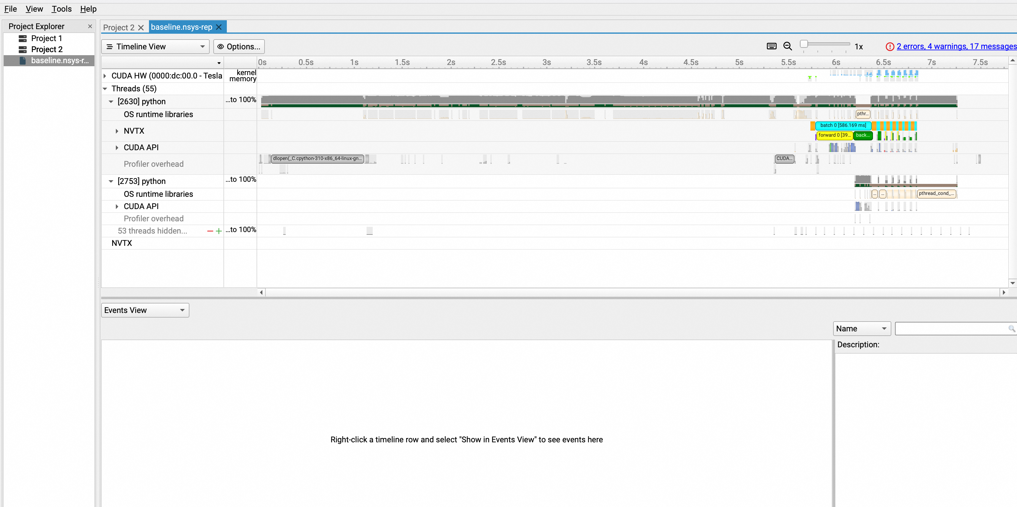
Files already downloaded and verified
Generating '/tmp/nsys-report-6673.qdstrm'
[1/1] [========================100%] baseline.nsys-rep
Generated:
    /root/baseline.nsys-rep
Import the baseline.nsys-rep file into the Nsight Systems UI to analyze the model. The following figure shows the initial view:
NoteIf you have not installed Nsight Systems, go to the NVIDIA Developer website and install the appropriate version for your system.
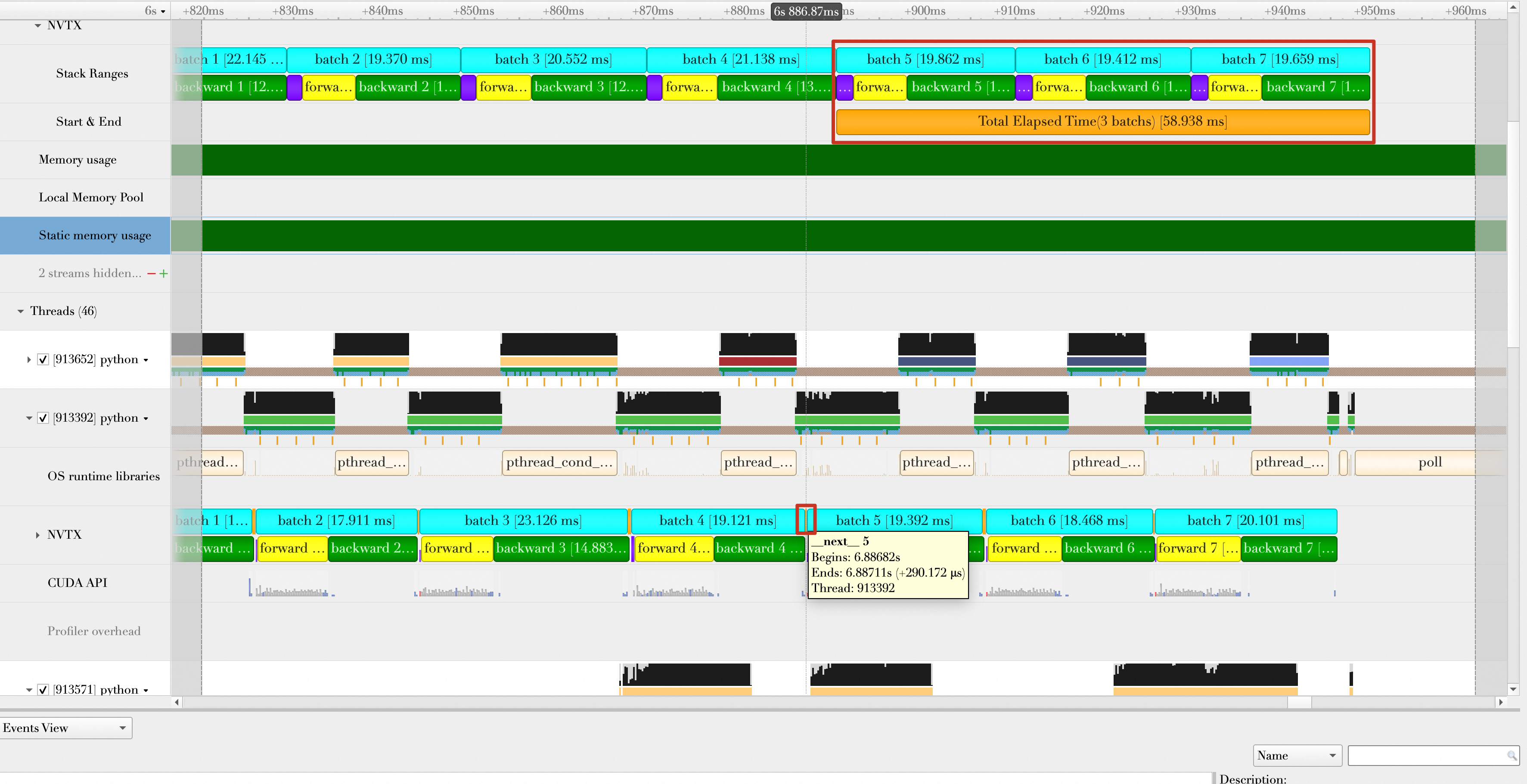
This topic references only the last 3 batches. The first 3 batches may be affected by initialization and warmup, which can lead to an inaccurate performance assessment. The following figure zooms in on the last 3 batches.
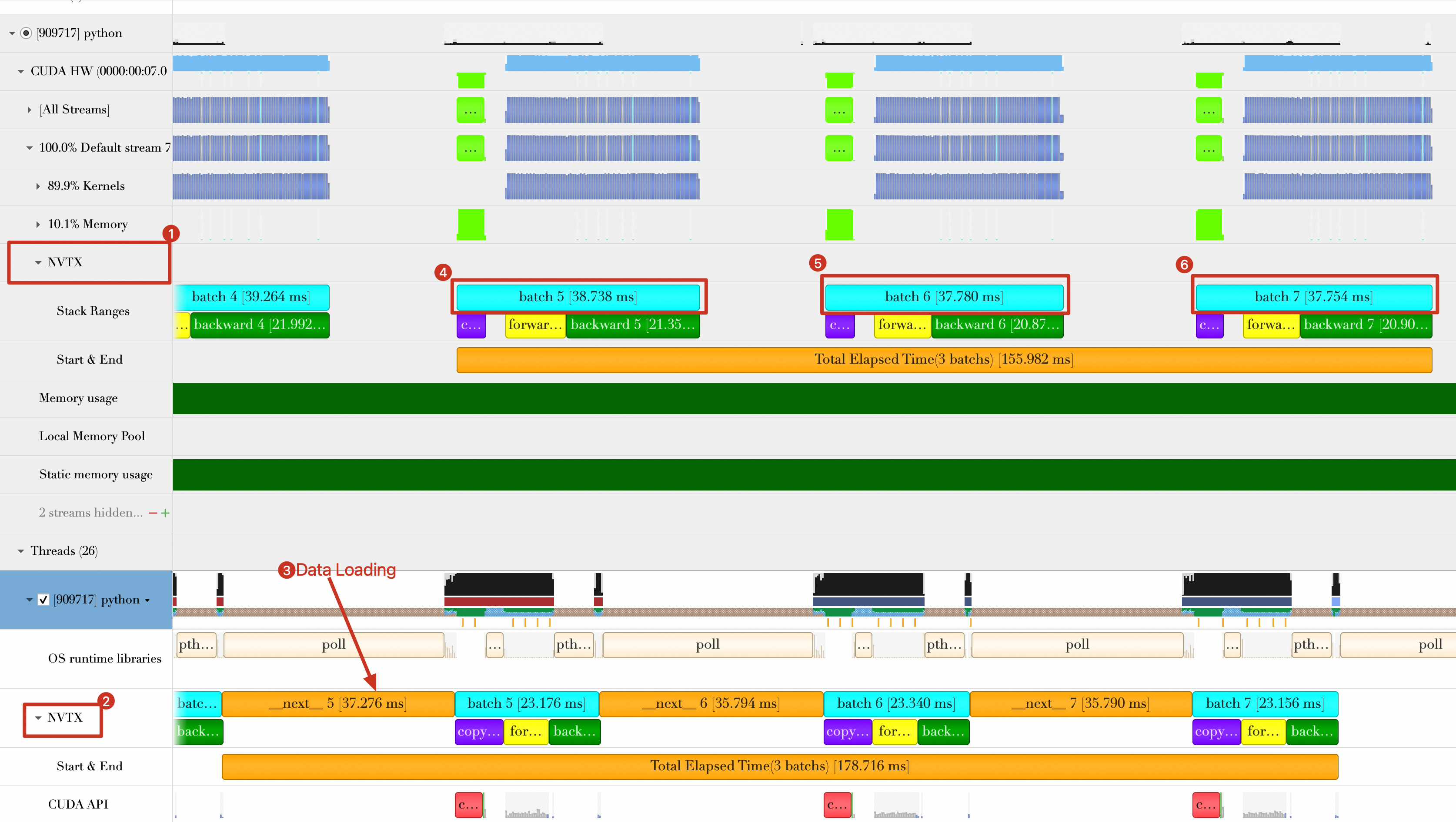
The figure shows two NVTX recordings of batch time: one in the CUDA stream (Default Stream, labeled 1) and one in the Python thread (labeled 2). Their batch time statistics, including
copy data,forward, andbackward, differ significantly. When you call CUDA APIs and run kernels on the GPU, rely on the NVTX data from the CUDA stream (labeled 1). Because batch transmission and GPU computing are asynchronous from the CPU's perspective, the Python thread statistics may be inaccurate.Batch data loading and batch computing, including batch transmission to the GPU, overlap. As shown in the figure, when loading Batch 6, the GPU is still computing Batch 5. Therefore, when you calculate the total duration of the 3 batches, do not count the overlapping time.
The baseline stage durations are as follows:
Stage duration
Time (ms)
Average data loading time (marked as __next__ in the figure)
(37.276 + 35.794 + 35.790) / 3 = 36.287
Average data transmission time (collapsed in the figure)
(4.39 + 4.363 + 4.317) / 3 = 4.357
Average batch processing time (includes data transmission, forward, and backward)
(38.738 + 37.78 + 37.754) / 3 = 38.091
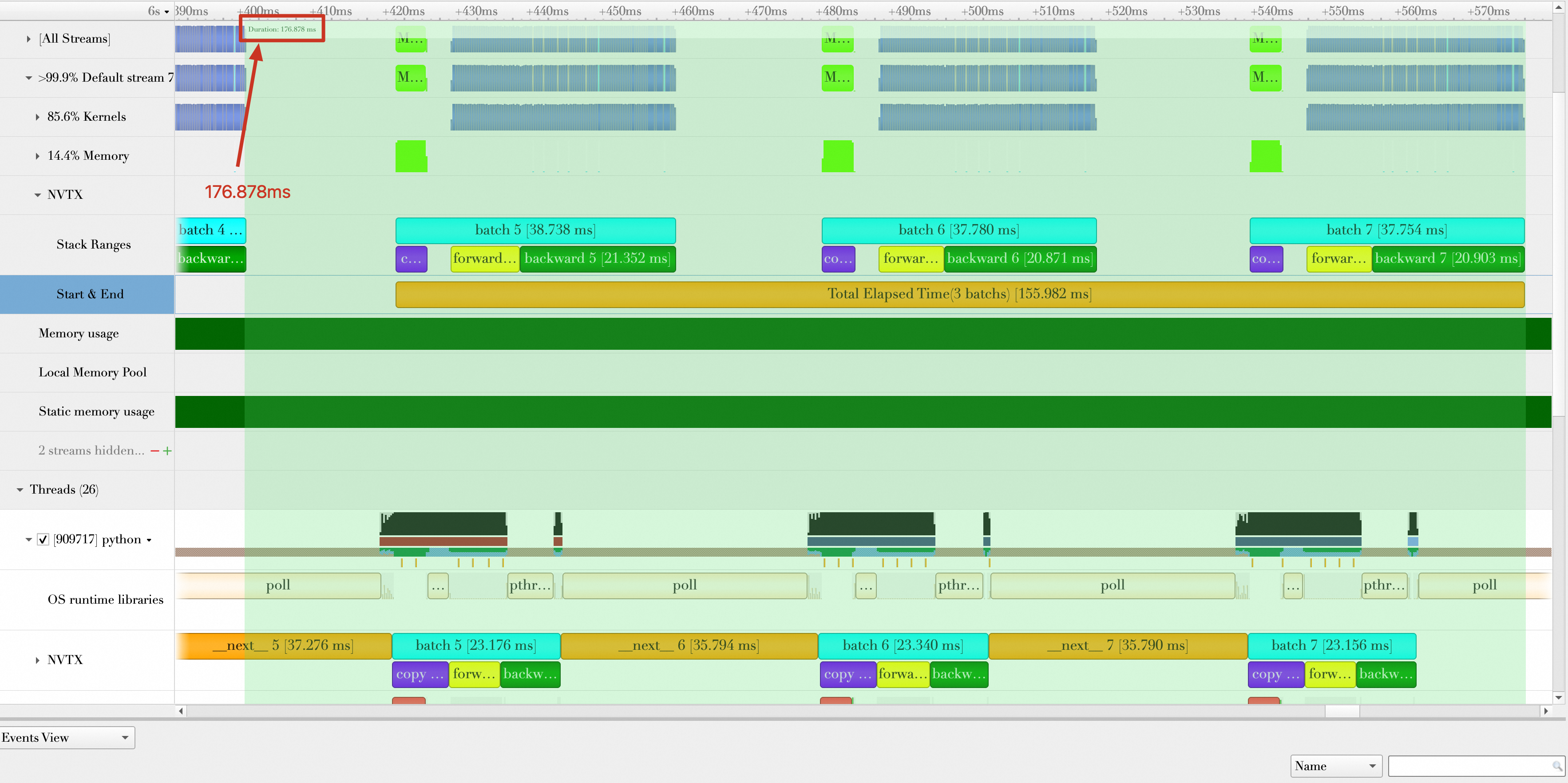
Total duration of 3 batches (from loading Batch 5 to completing Batch 7 computation)
176.878 ms
Average samples processed per second (samples/s)
32 (batch size) * 3 / (176.878 / 1000) = 542.746
Step 2: Optimize and analyze the model
Model optimization procedure
A single-machine deep learning training job consists of the following stages:
Data loading: Load data from a disk or other network storage to the host memory and preprocess it, such as by removing noise. This is the data loading stage.
Data transmission: Transfer data from the host memory to the GPU memory.
Training: GPU compute units, such as the CUDA Core and Tensor Core, use this data for training.

The following sections provide examples for each part.
Optimization 1: Reduce data loading time
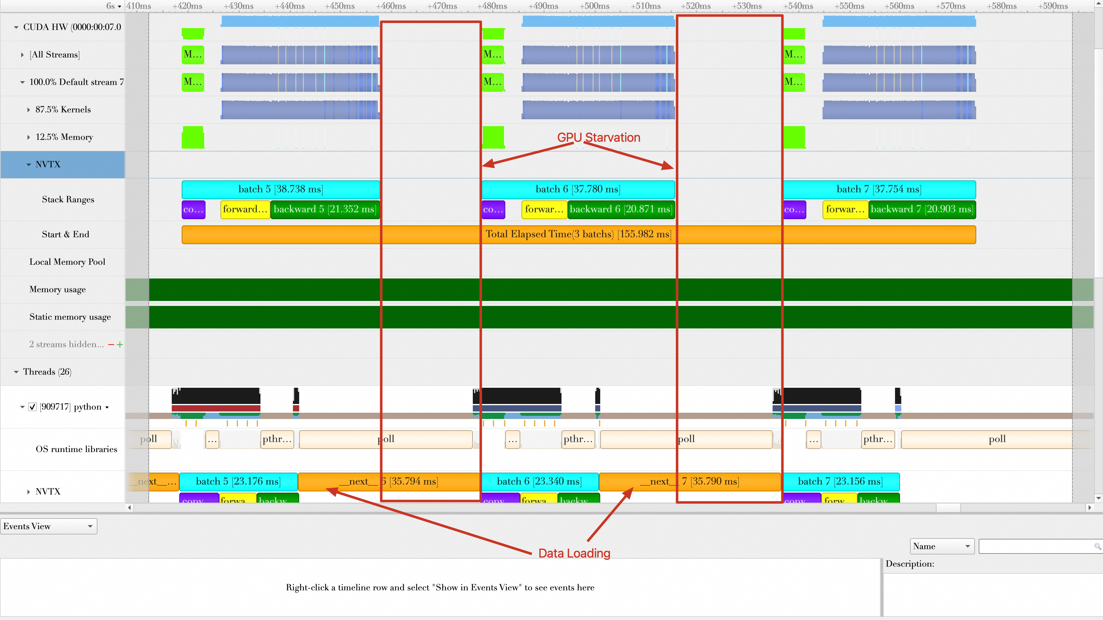
Reducing data loading time significantly improves training performance. If data loading takes longer than GPU training, the GPU may sit idle while waiting for data.
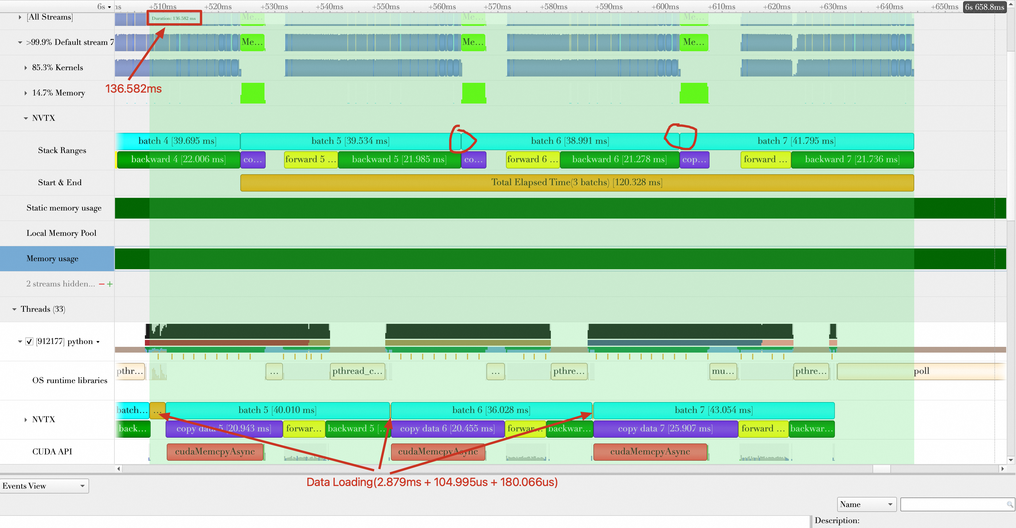
As shown in the following figure, the baseline, with no optimizations, has large gaps between batch computations. The root cause is the long batch data loading time. The GPU waits a long time for data before it can process each batch. Therefore, data loading becomes the training bottleneck.
The PyTorch DataLoader supports multiple workers (multi-process) to load mini-batch data simultaneously. You can modify the train_loader parameter in main.py to use 8 workers for data loading.
train_loader = torch.utils.data.DataLoader(train_set,num_workers=8, batch_size=32, shuffle=True)After you rerun the script, the gaps between batches disappear, and the data loading time drops significantly. The average loading time for three batches is (2.879 ms + 104.995 μs + 180.066 μs) / 3 = 1.055 ms. The number of samples processed per second (samples/s) is 32 * 3 / (120.328 / 1000) = 797.819. You can ignore the data loading time because it overlaps with GPU computing. The performance improves by (797.819 - 542.746) / 542.746 * 100% = 47.00% compared to the baseline.
Optimization 2: Reduce data transmission time
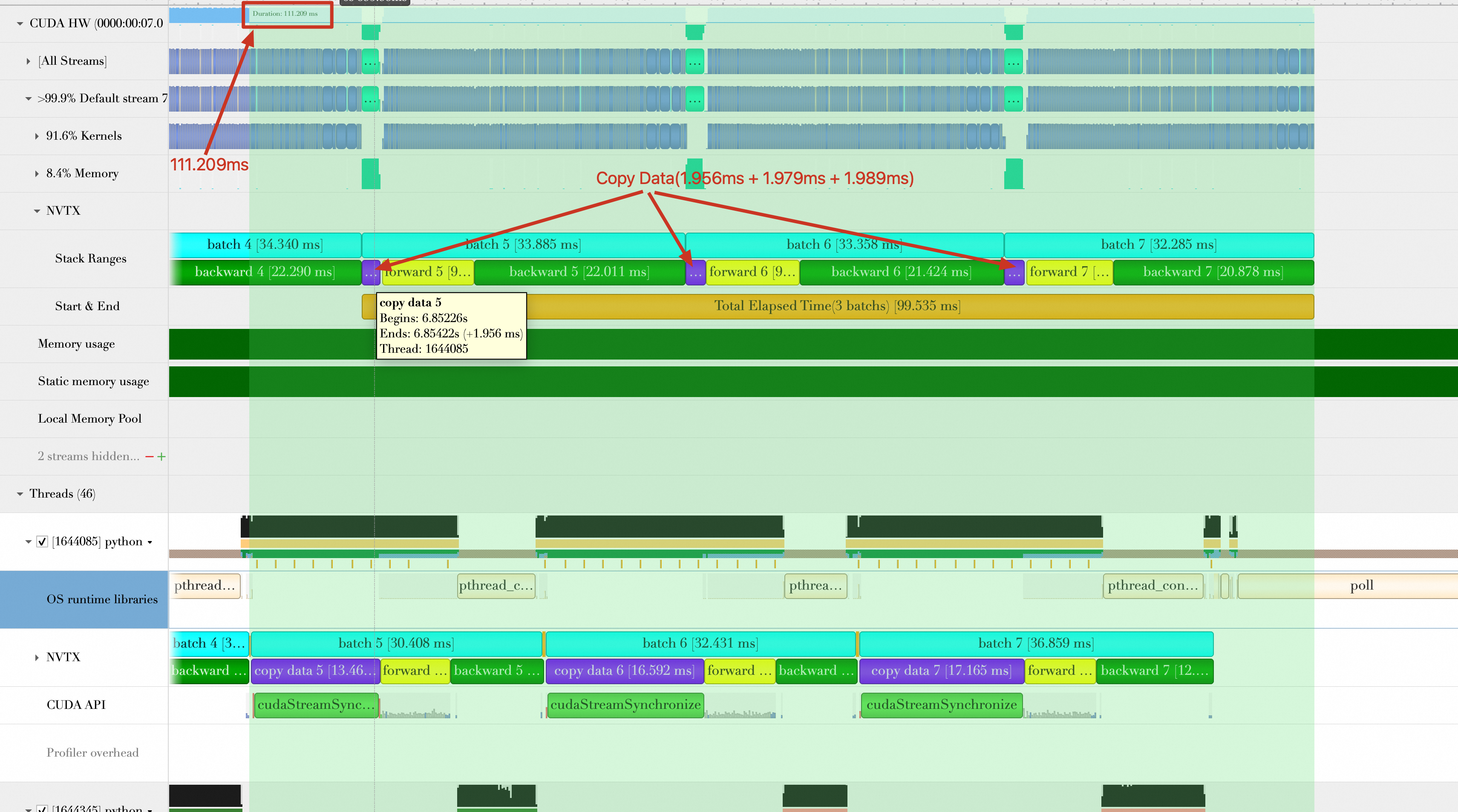
With 8 workers set, you can continue to optimize the sample model. The previous analysis showed that the average data transmission time was 4.357 ms. You can enable Pin Memory to reduce this time.
PyTorch supports storing loaded data directly in Pin Memory. You can modify the train_loader parameter in main.py to enable Pin Memory.
train_loader = torch.utils.data.DataLoader(train_set,num_workers=8, batch_size=32,pin_memory=True, shuffle=True)After you rerun the script, the average data transmission time is (1.956 + 1.979 + 1.989) / 3 = 1.975 ms, which reduces the baseline time by 4.357 ms - 1.975 ms = 2.382 ms. The total duration drops to 99.535 ms. The average number of samples processed per second (samples/s) is:
32 * 3 /(99.535 / 1000) = 964.485. The performance improves by (964.485 - 797.819) / 797.819 * 100% = 20.89%.
Optimization 3: Fully overlap data loading and data computing
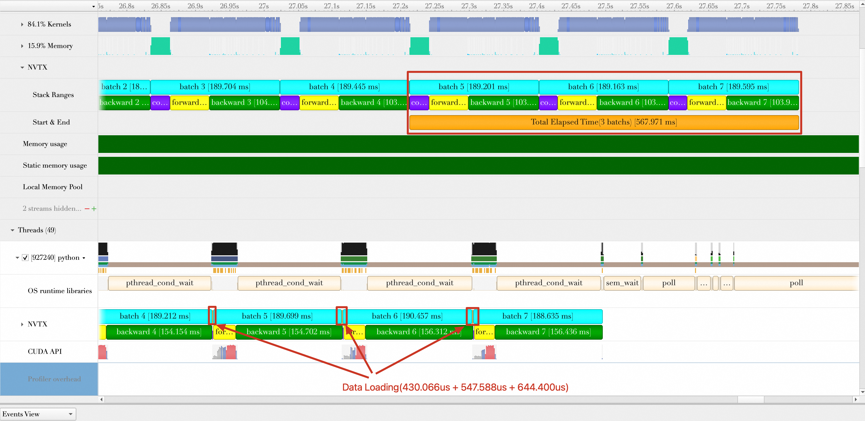
After reducing the data transmission time, you can seek further optimization. Analyzing the Pin Memory-enabled timeline shows that batch loading and batch computing, including transmission, overlap, but each batch load overlaps with only one batch compute. As shown in the figure, Batch 5 loading overlaps with Batch 4 computing, Batch 6 with Batch 5, and Batch 7 with Batch 6. Cases where Batch 6 and 7 loading overlap with Batch 5 computing do not occur. In addition, after each data loading operation, cudaStreamSynchronize forces a CPU-GPU sync, which is unnecessary for batch computing.
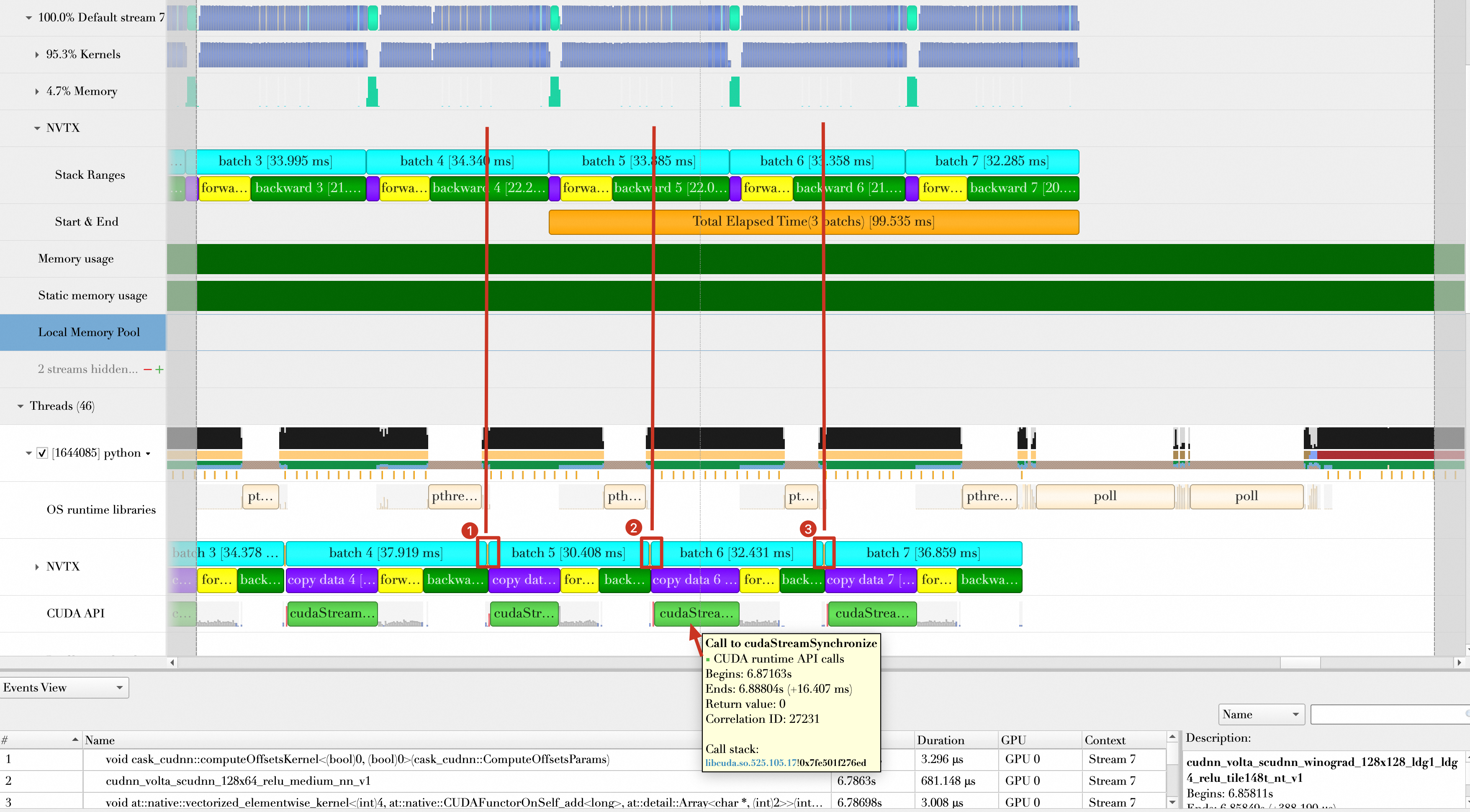
This sync comes from the following line of code:
inputs, labels = data[0].to(device=device), data[1].to(device=device)By default, the to function executes cudaStreamSynchronize after each host-to-GPU data transfer. However, the to function also supports a non-blocking mode (asynchronous operation) using the non_blocking=True parameter:
inputs, labels = data[0].to(device=device,non_blocking=True), data[1].to(device=device,non_blocking=True)In non-blocking mode, the GPU data transmission is queued at the end of the CUDA stream without blocking the CPU. The CPU can then continue with subsequent tasks without waiting for the transmission to complete.
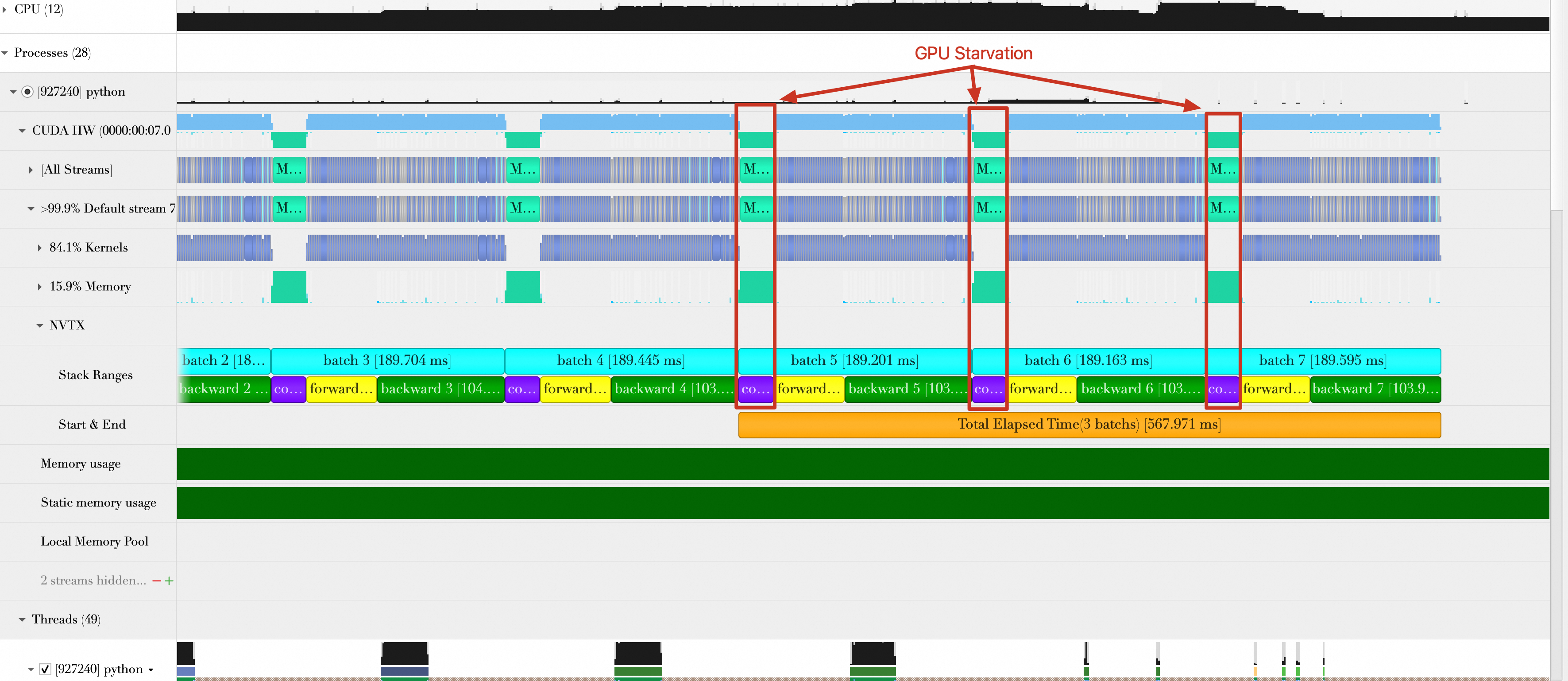
After you modify the code and rerun the script, the results are as follows.
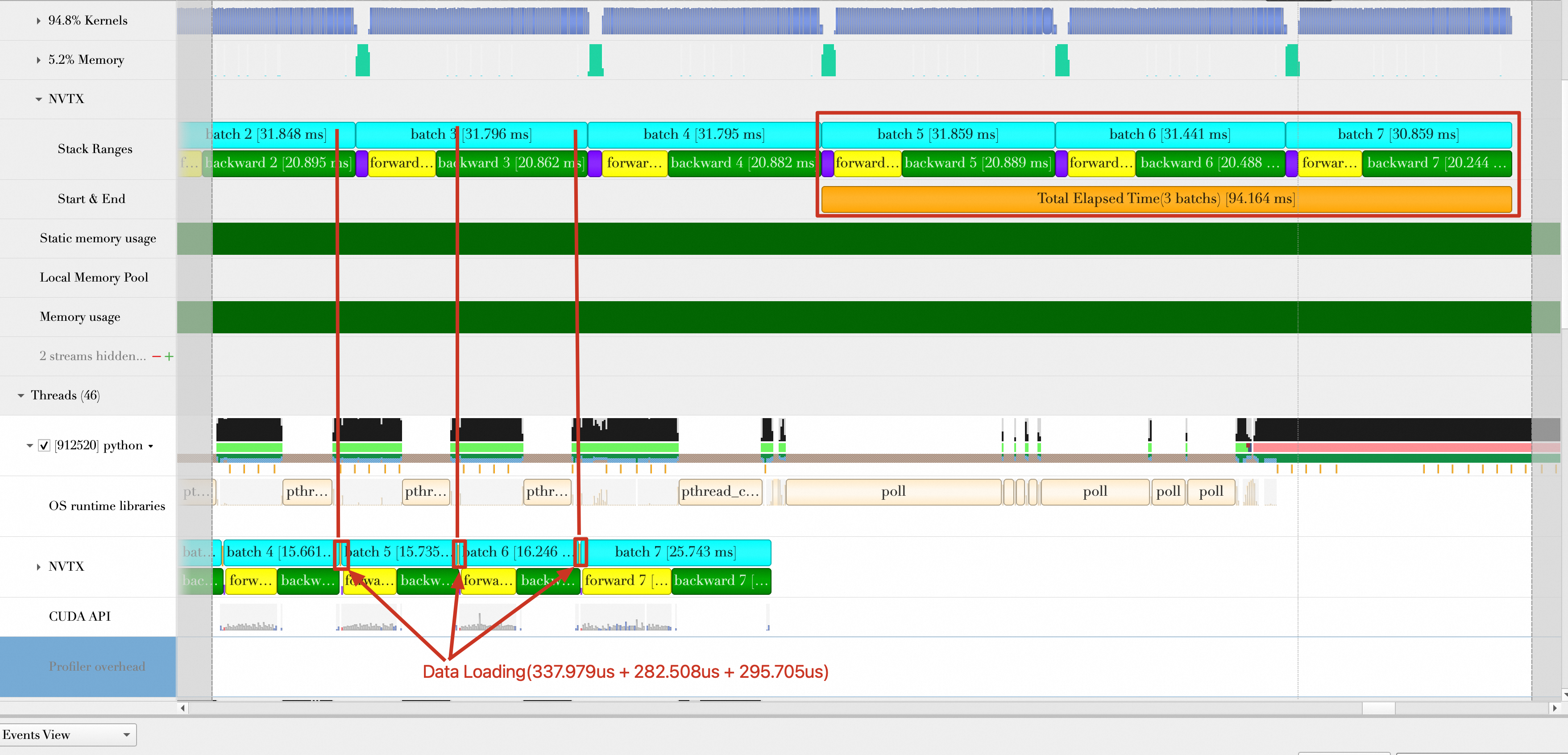
The figure shows the following:
When the GPU computes Batch 3, the CPU has already finished loading the data for Batch 5, 6, and 7. This achieves a full overlap between batch loading and computing.
The loading for Batch 5, 6, and 7 is fully hidden within the computing for Batch 2, 3, and 4. Their loading time is negligible.
The number of samples processed per second (samples/s) is 32 × 3 / (94.164 / 1000) = 1019.498. The performance improves by (1019.498 - 964.485) / 964.485 × 100% = 5.7% compared to Optimization 2.
Optimization 4: Automatic Mixed Precision
The previous steps optimized data loading and transmission. This section focuses on reducing the GPU batch computing time.
PyTorch supports mixed-precision training through Automatic Mixed Precision (AMP). In AMP mode, some tensors are automatically converted to low-precision 16-bit floating-point numbers and run on GPU Tensor Cores. This reduces GPU memory usage and computing time.
You can modify the code as shown below to enable AMP. In a production environment, a full AMP implementation may require gradient scaling, which this demo omits. For more information about correct usage, see the AMP documentation.
# train step
def train(data):
    # Omit other code
    # Enable amp
    with torch.autocast(device_type='cuda', dtype=torch.float16):
        outputs = model(inputs)
        loss = criterion(outputs, labels)
    # Omit other code
With AMP enabled, the batch computing time drops to 58.938 ms. The average number of samples processed per second is 32 × 3 / (58.938 /1000) = 1628.83. The performance improves by (1628.83 - 1019.498) / 1019.498 × 100% = 59.77%.
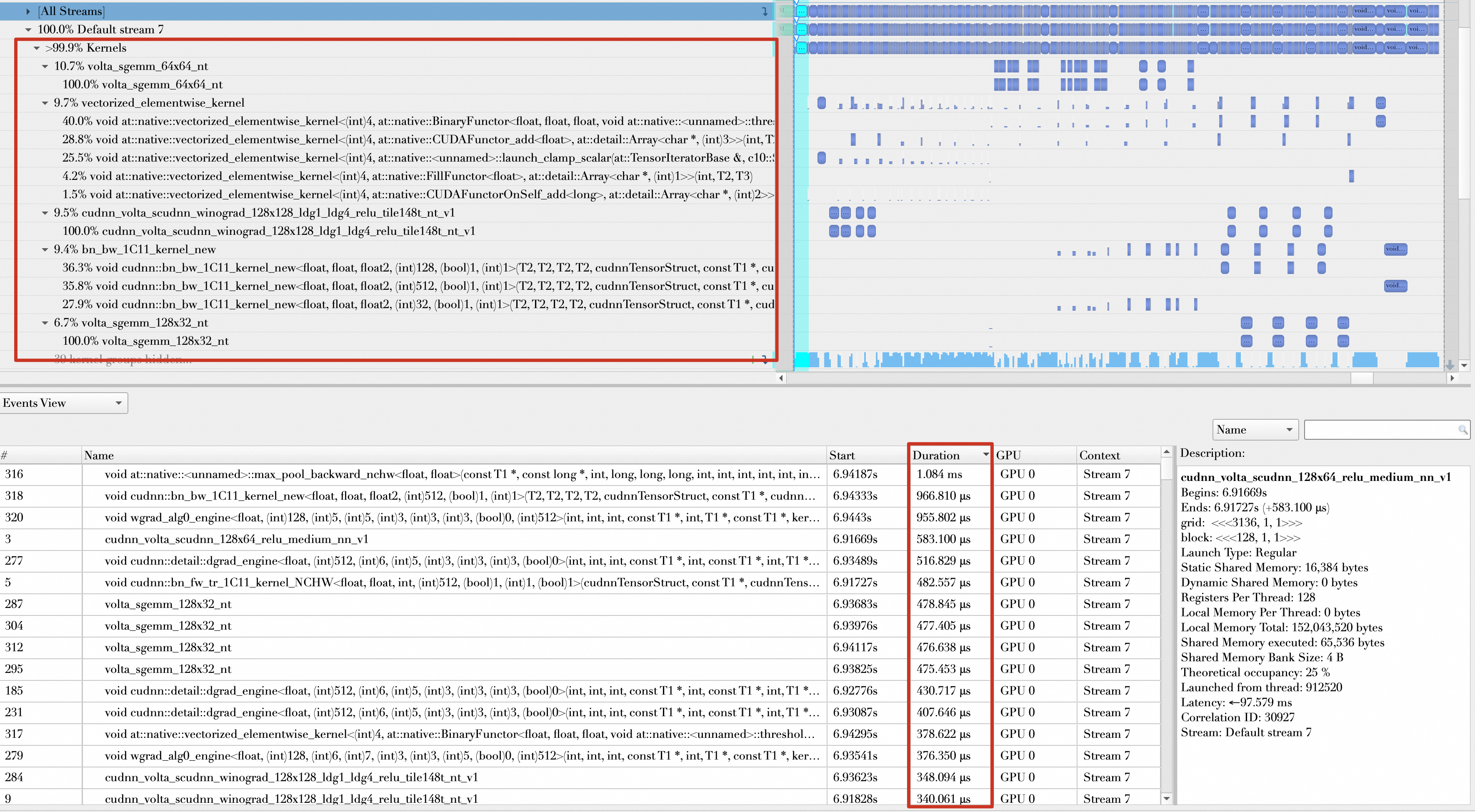
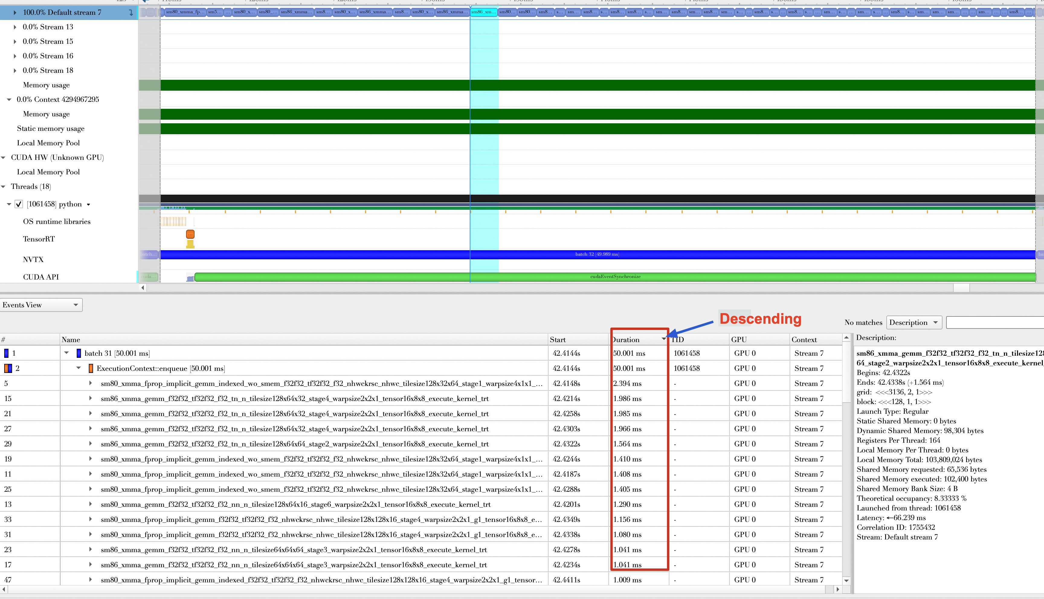
Inspecting the forward and backward passes of a batch shows the kernel composition. Before AMP was enabled, operations mostly used float32 data. If you sort the kernels by descending execution time, the top kernels range from 300 μs to 1 ms.
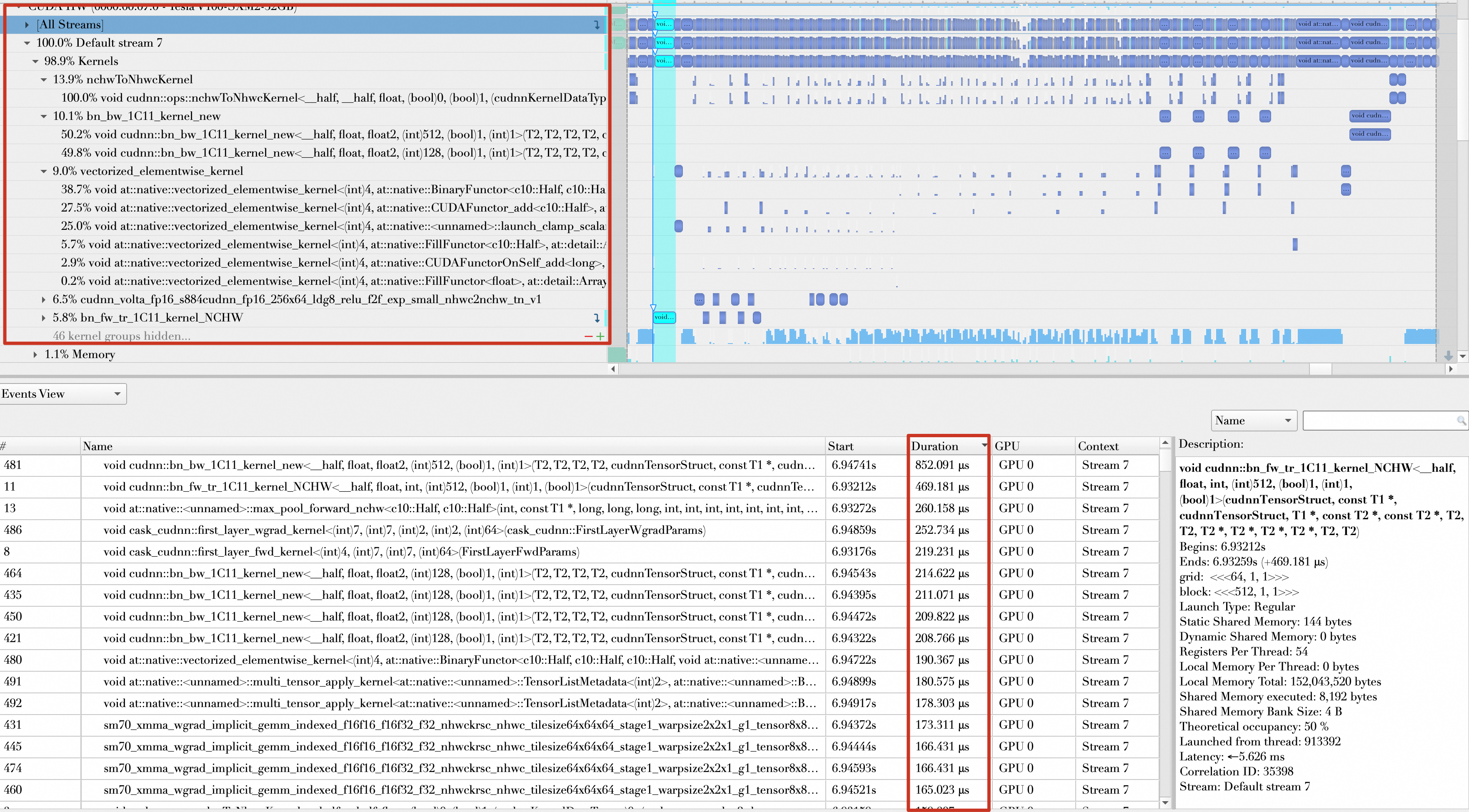
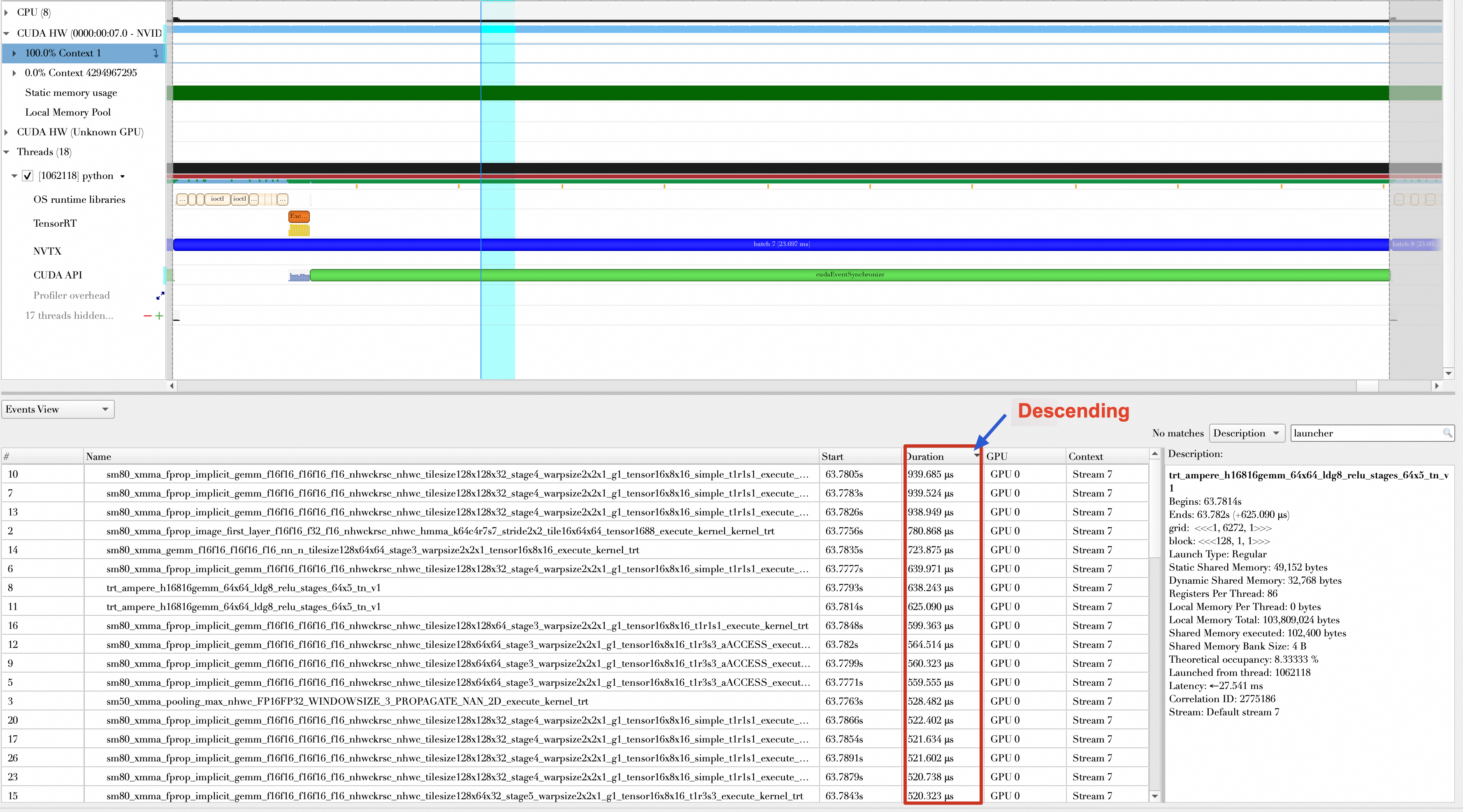
After AMP is enabled, most operations use float16 data, and the top kernels range from 100 μs to 300 μs.
Optimization 5: Increase batch size
Increasing the batch size can boost the number of samples processed per second. However, you must consider GPU memory availability and the impact of large batches on loss values.
You can modify the code as shown below to adjust the batch size from 32 to 512.
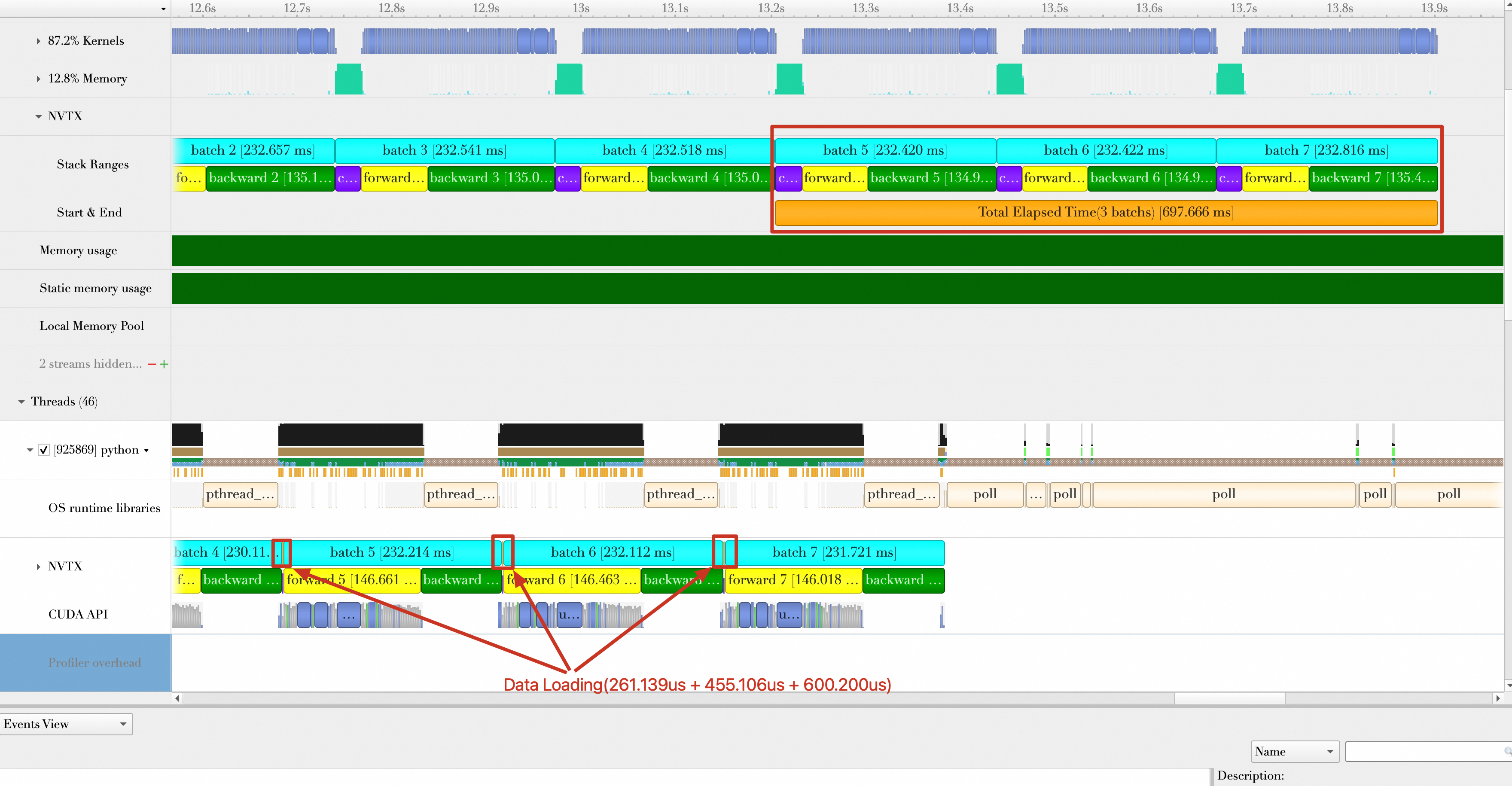
train_loader = torch.utils.data.DataLoader(train_set,num_workers=8, batch_size=512,pin_memory=True, shuffle=True)After running the script, the total duration is 697.666 ms. The average number of samples processed per second (samples/s) is 512 × 3 / (697.666 / 1000) = 2201.627. The performance improves by (2201.627 - 1628.83) / 1628.83 × 100% = 35.17%.
Optimization 6: Model compilation
By default, PyTorch uses just-in-time compilation. You can use the PyTorch compile API to compile the model into graph mode.
You can modify the code as follows:
model = torchvision.models.resnet18(weights='IMAGENET1K_V1').cuda(device)
model = torch.compile(model)
After running the script, the total duration is 567.971 ms. The average number of samples processed per second is 512 × 3 / (567.971 / 1000) = 2704.36. The performance improves by (2704.36 - 2201.627) / 2201.627 × 100% = 22.83%.
Note that model compilation may not help in small-batch scenarios.
Optimization 7: Overlap batch transmission and batch computing
Batch transmission and computing execute sequentially. Batch computing starts only after the transmission is complete. During transmission, the GPU is idle. With larger batch sizes, the transmission time becomes significant compared to the computing time.
Normally, batch computing requires the data to be completely transmitted to the GPU first. Starting the computation during transmission yields incorrect results. However, using a pipeline approach, if the batch computing time exceeds the transmission time, you can start transmitting Batch 2 while computing Batch 1, and transmit Batch 3 while computing Batch 2. This approach hides the transmission time within the computing time.
Single-stream execution cannot achieve this overlap. However, PyTorch lets you create multiple streams in addition to the default stream. The full code is as follows:
import nvtx  # Import nvtx package
import torch
import torch.nn
import torch.optim
import torch.profiler
import torch.utils.data
import torchvision.datasets
import torchvision.models
import torchvision.transforms as T

transform = T.Compose([
    T.Resize(224),
    T.ToTensor(),
    T.Normalize((0.5, 0.5, 0.5), (0.5, 0.5, 0.5))])
train_set = torchvision.datasets.CIFAR10(root='./data', train=True, download=True, transform=transform)
train_loader = torch.utils.data.DataLoader(train_set, num_workers=8, batch_size=512, pin_memory=True, shuffle=True)

device = torch.device("cuda:0")
model = torchvision.models.resnet18(weights='IMAGENET1K_V1').cuda(device)
model = torch.compile(model)
criterion = torch.nn.CrossEntropyLoss().cuda(device)
optimizer = torch.optim.SGD(model.parameters(), lr=0.001, momentum=0.9)

def train(model, device, train_loader, optimizer, criterion):
	model.train()
	dl = iter(train_loader)
	transfered_data = []
	# Create a new stream
	s = torch.cuda.Stream()

	def prepare_batch(batch_idx):
		nvtx.push_range("__next__ " + str(batch_idx), color="orange")
		(inputs, labels) = next(dl)
		# Transmit data in the new stream
		nvtx.pop_range()
		nvtx.push_range("cpy " + str(batch_idx), color="rapids")
		with torch.cuda.stream(s):
			inputs, labels = inputs.to(device=device, non_blocking=True), labels.to(device=device, non_blocking=True)
		nvtx.pop_range()
		return (inputs, labels)

	def batch_compute(batch_idx, data):
		nvtx.push_range("batch " + str(batch_idx), color="cyan")
		nvtx.push_range("forward " + str(batch_idx), color="yellow")
		with torch.autocast(device_type='cuda', dtype=torch.float16):
			outputs = model(data[0])
			loss = criterion(outputs, data[1])
		nvtx.pop_range()
		nvtx.push_range("backward " + str(batch_idx), color="green")
		optimizer.zero_grad()
		loss.backward()
		optimizer.step()
		nvtx.pop_range()
		torch.cuda.current_stream().wait_stream(s)
		nvtx.pop_range()

	batch_idx = 0
	tet = None
	while True:
		try:
			if batch_idx == 6:
				tet = nvtx.start_range(message="Total Elapsed Time(3 batchs)", color="orange")
			if batch_idx >= 8:
				break
			data = prepare_batch(batch_idx)
			transfered_data.append(data)
			# Skip computation when batch_idx is 0
			# Each loop requires the default stream to wait for the new stream's data transmission,
			# ensuring data readiness for the next batch computation.
			if batch_idx > 0:
				batch_compute(batch_idx - 1, transfered_data[batch_idx - 1])
			else:
				torch.cuda.current_stream().wait_stream(s)
			batch_idx += 1
		except StopIteration:
			nvtx.pop_range()
			break
	batch_compute(batch_idx - 1, transfered_data[batch_idx - 1])
	nvtx.end_range(tet)


train(model, device, train_loader, optimizer, criterion)
The following figure shows the results of the run. The transmission for Batches 2 to 7 overlaps with the computation for Batches 1 to 4. The transmission for Batches 0 and 1 is not shown due to space limitations. To ensure correct results, the data transmission for each batch is completed before its computation begins. For example, the transmission for Batch 4 occurs during the computation for Batch 2.
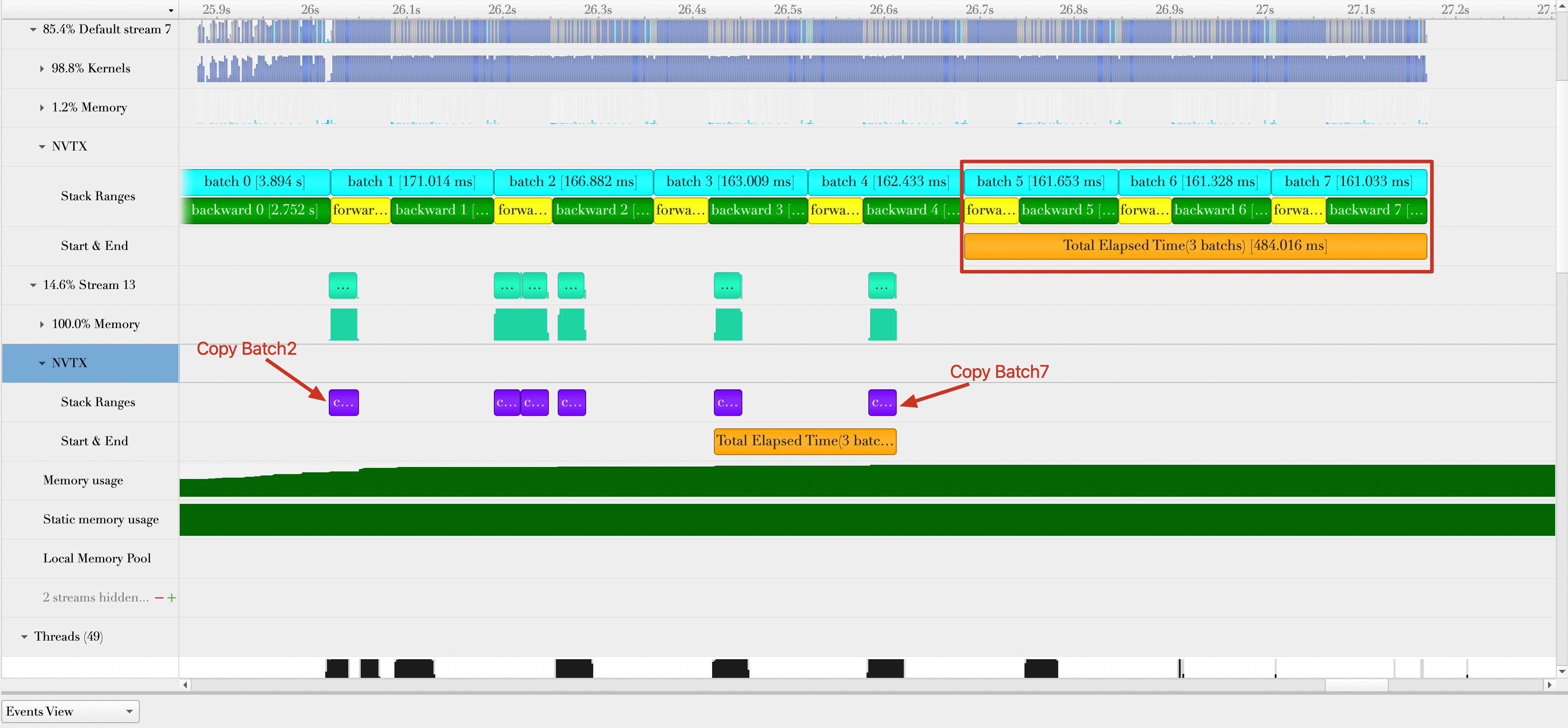
The total duration is 484.016 ms. The average number of samples processed per second is 3173.449 (512 × 3 ÷ (484.016 ÷ 1000)), which is a 17.35% performance improvement ((3173.449 - 2704.36) ÷ 2704.36 × 100%).
Note that overlapping computation and data transmission increases GPU memory usage. In this example, when computing Batch 5, all batches reside in GPU memory.
Summary
Performance gains from each optimization:
Stage | Average samples processed per second (samples/s) | Performance improvement vs. previous optimization (%) |
No optimization: Baseline | 542.746 | - |
Optimization 1: Set DataLoader workers to 8 | 797.819 | 47.00% |
Optimization 2: Enable Pin Memory | 964.485 | 20.89% |
Optimization 3: Fully overlap data loading and batch computing | 1019.498 | 5.7% |
Optimization 4: Automatic Mixed Precision | 1628.83 | 59.77% |
Optimization 5: Increase batch size | 2201.627 | 35.17% |
Optimization 6: Model compilation | 2704.36 | 22.83% |
Optimization 7: Overlap batch transmission and batch computing | 3173.449 | 17.35% |
Inference scenarios
Many inference frameworks support model optimization. This section uses a TensorRT-optimized ResNet-50 model to demonstrate performance analysis with Nsight Systems in inference scenarios.
Step 1: Create a sample model
Inside the PyTorch container, create a main.py file and copy the following content into it.
The main.py file integrates PyTorch models with TensorRT to accelerate inference and provides basic model loading, prediction, and performance evaluation features.
Note that the model loading path is model/vision-v0.10.0 in the current directory.
#!/usr/bin/env python
# -*- coding: UTF-8 -*-
import argparse
import torch
import torchvision
from PIL import Image
import matplotlib.pyplot as plt
import json
from torchvision import models as M
from torchvision import transforms

import numpy as np
import time
import torch.backends.cudnn as cudnn
import torch_tensorrt
import nvtx

cudnn.benchmark = True

def load_model():
    torch.hub._validate_not_a_forked_repo=lambda a,b,c: True
    weights=M.ResNet50_Weights.IMAGENET1K_V1
    #resnet50_model = torch.hub.load('pytorch/vision:v0.10.0', 'resnet50',force_reload=True,skip_validation=True, weights=weights)
    resnet50_model = torch.hub.load('model/vision-v0.10.0', 'resnet50',source='local', weights=weights)
    resnet50_model.load_state_dict(torch.load('./resnet50-0676ba61.pth'))
    return resnet50_model


def rn50_preprocess():
    preprocess = transforms.Compose([
        transforms.Resize(256),
        transforms.CenterCrop(224),
        transforms.ToTensor(),
        transforms.Normalize(mean=[0.485, 0.456, 0.406], std=[0.229, 0.224, 0.225]),
    ])
    return preprocess

def load_labels():
    # loading labels
    with open("./data/imagenet_class_index.json") as json_file:
        d = json.load(json_file)

# decode the results into ([predicted class, description], probability)
def predict(img_path, model,labels):
    model.eval()
    img = Image.open(img_path)
    preprocess = rn50_preprocess()
    input_tensor = preprocess(img)
    input_batch = input_tensor.unsqueeze(0) # create a mini-batch as expected by the model

    # move the input and model to GPU for speed if available
    if torch.cuda.is_available():
        input_batch = input_batch.to('cuda')
        model.to('cuda')

    with torch.no_grad():
        output = model(input_batch)
        # Tensor of shape 1000, with confidence scores over Imagenet's 1000 classes
        sm_output = torch.nn.functional.softmax(output[0], dim=0)

    ind = torch.argmax(sm_output)
    return labels[str(ind.item())], sm_output[ind] #([predicted class, description], probability)

def benchmark(model, input_shape=(1024, 1, 224, 224), dtype='fp32', nwarmup=50, nruns=10000):
    model.eval()
    input_data = torch.randn(input_shape)
    input_data = input_data.to("cuda")
    if dtype=='fp16':
        input_data = input_data.half()

    print("Warm up ...")
    with torch.no_grad():
        for _ in range(nwarmup):
            features = model(input_data)
    torch.cuda.synchronize()
    print("Start timing ...")
    timings = []
    e = torch.cuda.Event(enable_timing=False)
    with torch.no_grad():
        for i in range(1, nruns+1):
            start_time = time.time()
            nvtx.push_range("batch " + str(i),"blue")
            e.record()
            features = model(input_data)
            e.synchronize()
            nvtx.pop_range()
            end_time = time.time()
            timings.append(end_time - start_time)
            if i%10==0:
                print('Iteration %d/%d, ave batch time %.2f ms'%(i, nruns, np.mean(timings)*1000))

    print("Input shape:", input_data.size())
    print("Output features size:", features.size())
    print('Average batch time: %.2f ms'%(np.mean(timings)*1000))


def main():
    # Training settings
    parser = argparse.ArgumentParser(description='PyTorch RESNET Example')
    parser.add_argument('--enable-tensorrt', action='store_true', default=False,
                        help='Enable tensorrt to optimize model')
    parser.add_argument('--precision', type=str, default='fp32', metavar='N',
                        help='specify the precision when tensorrt is enabled,value in [fp32,fp16] (default: fp32)')
    args = parser.parse_args()
    model = load_model()
    model = model.eval().to("cuda")
    optimized_model = model
    dtype = "fp32"
    if args.enable_tensorrt:
        if args.precision == "fp32":
           optimized_model = torch_tensorrt.compile(
                                model, inputs = [torch_tensorrt.Input((128, 3, 224, 224), dtype=torch.float32)],
                                enabled_precisions = torch.float32, # Run with FP32
                                workspace_size = 1 << 22,
                            )
        elif args.precision == "fp16":
            optimized_model = torch_tensorrt.compile(
                                model, inputs = [torch_tensorrt.Input((128, 3, 224, 224), dtype=torch.half)],
                                enabled_precisions = {torch.half}, # Run with FP16
                                workspace_size = 1 << 22
                            )
            dtype = "fp16"
    benchmark(optimized_model, input_shape=(128, 3, 224, 224),dtype=dtype, nruns=100)

if __name__ == '__main__':
    main()
Step 2: Generate profiling reports
You can generate profiling reports for the following three scenarios and then compare the model optimization effects using the Nsight Systems report files.
No model optimization | Optimize model with TensorRT without quantization | Optimize model with TensorRT and enable quantization |
Run the following command to generate an Nsight Systems report file. | You can optimize the model with TensorRT without quantization. In this case, the model weights and activation precision remain FP32. Run the following command to generate an Nsight Systems report file. | You can optimize the model with TensorRT and enable quantization. In this case, the model weights and activation precision use FP16. Run the following command to generate an Nsight Systems report file. |
After you run these commands, three Nsight Systems report files appear in the current directory:
resnet-50-none-tensorrt.nsys-rep
resnet-50-tensorrt-fp32.nsys-rep
resnet-50-tensorrt-fp16.nsys-rep
Import these files into the Nsight Systems UI to start profiling.
Step 3: View profiling reports
Before you view and analyze the profiling reports, it is helpful to understand the optimizations that TensorRT provides. According to the official TensorRT documentation, TensorRT provides the following capabilities:
Layer and Tensor Fusion: During inference, many short-running kernels are launched on the GPU. Launching each kernel takes a significant amount of time. If there are many kernels, the launch overhead becomes dominant. TensorRT fuses multiple kernels into a single kernel to solve this issue.
Weight and Activation Precision Calibration: Most deep learning frameworks use FP32 tensors during neural network training. TensorRT automatically converts some FP32 tensors to FP16 or INT8 to reduce GPU memory usage and computing time while it minimizes accuracy loss.
Kernel Auto-Tuning: Automatically calculates the optimal grid and block sizes during a kernel launch to maximize GPU SM occupancy.
Dynamic Tensor Memory: Assigns GPU memory to each tensor only during its usage period. This avoids repeated allocations, reduces the memory footprint, and improves reuse efficiency.
Multi-Stream Execution: Launches multiple CUDA streams for concurrent task execution.
You can now observe these TensorRT capabilities in the Nsight Systems UI.
Layer & Tensor Fusion
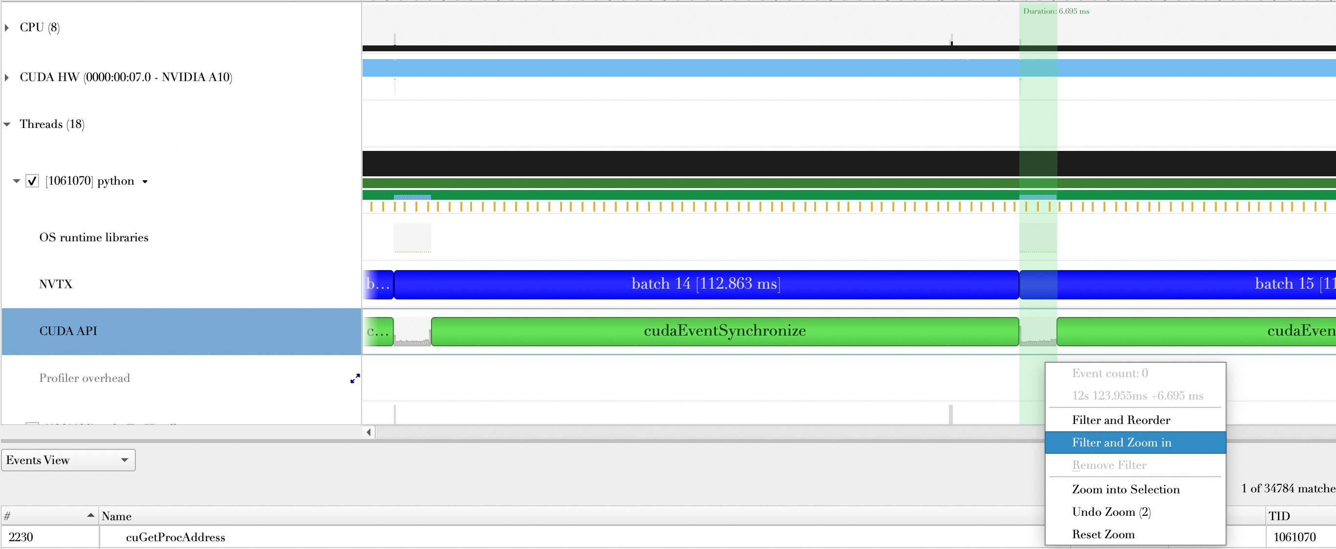
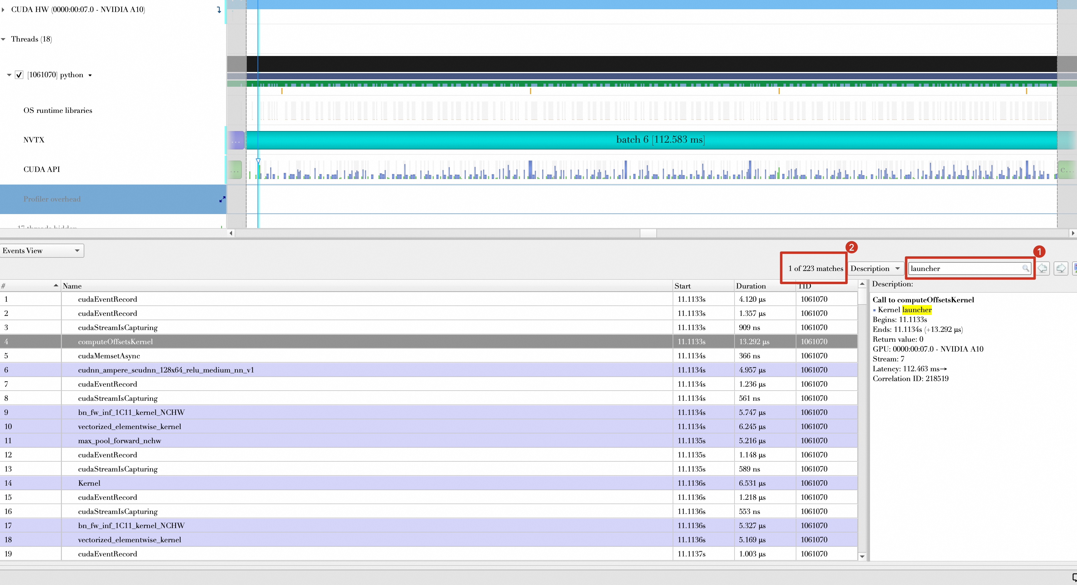
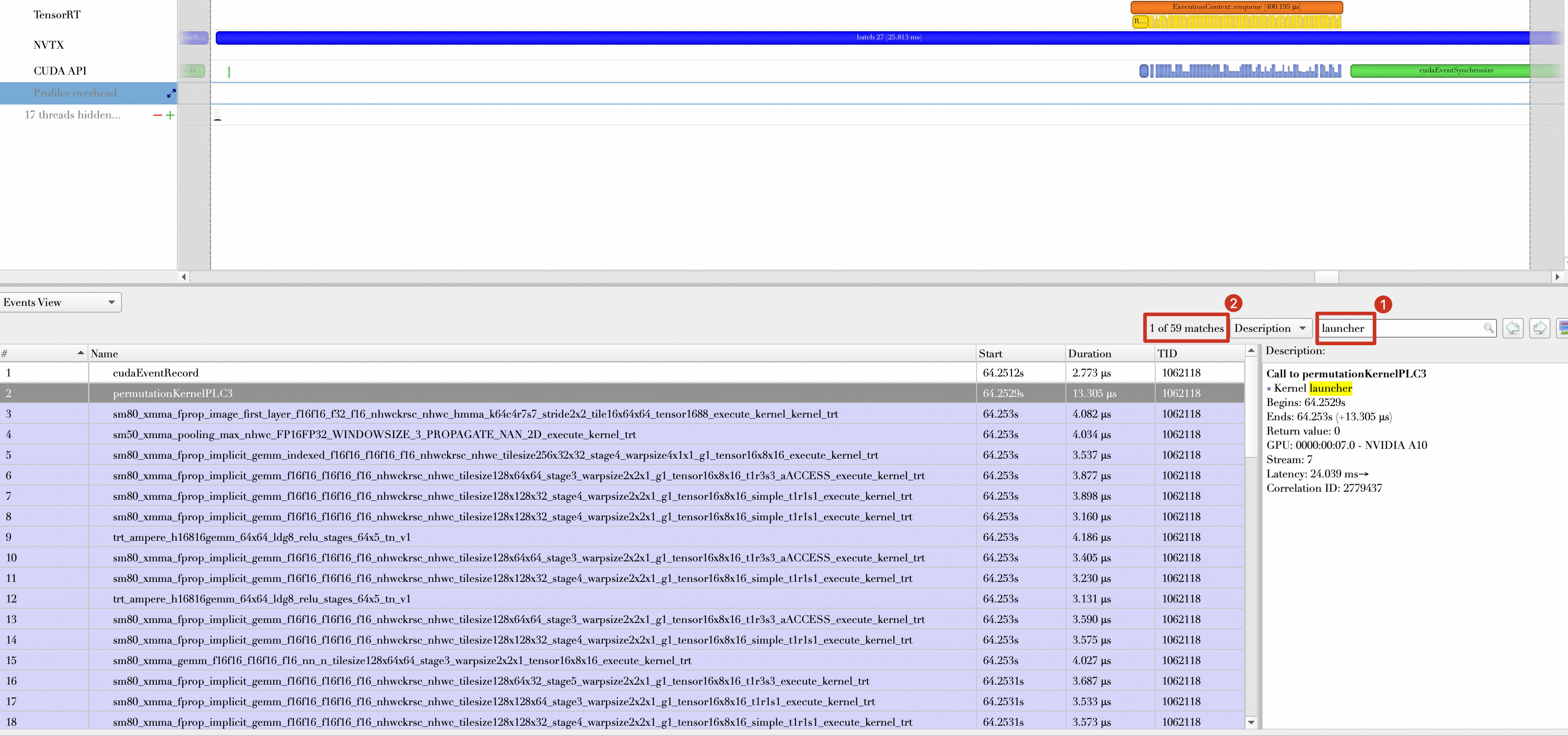
You can check how many kernel launches occur per batch computation.
No model optimization | Optimize model with TensorRT without quantization | Optimize model with TensorRT and enable quantization |
|
|
|
Conclusion
Comparison item | Without TensorRT | With TensorRT (quantization disabled) | With TensorRT (quantization enabled) |
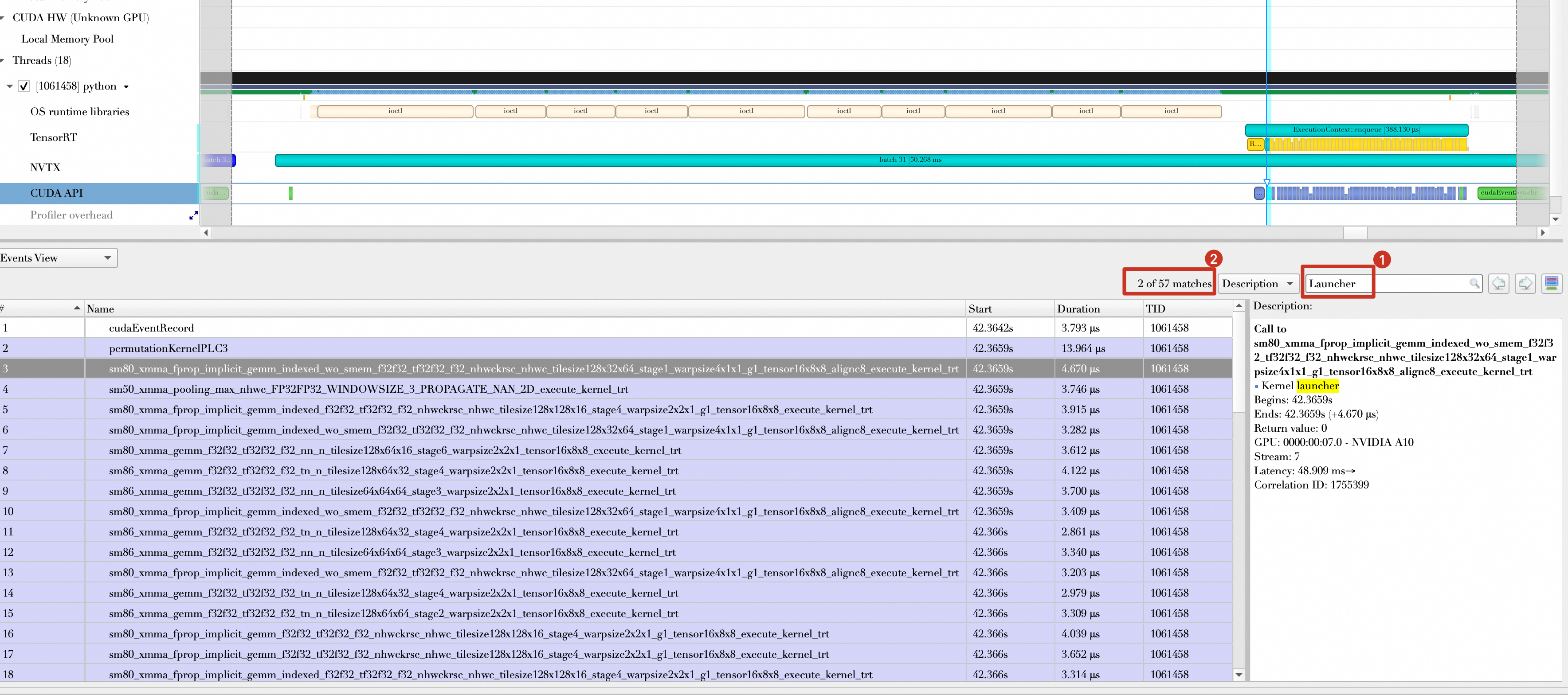
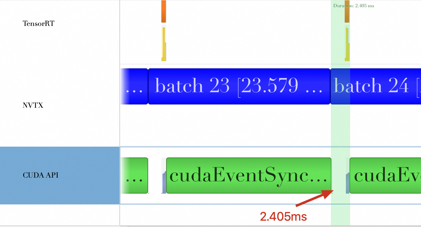
Kernel launches per batch computation | 233 | 57 | 59 |
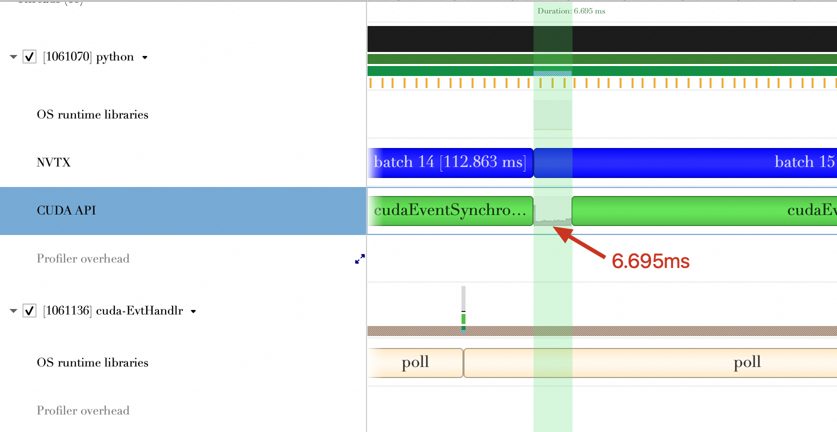
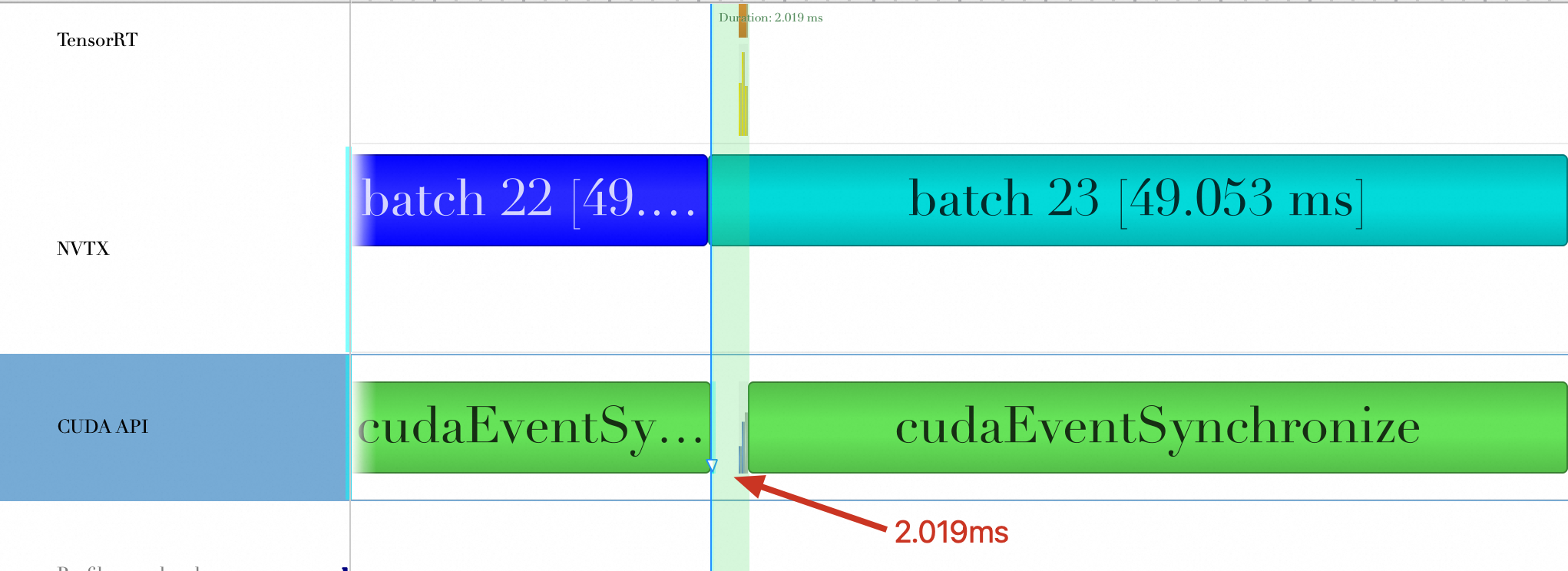
Time spent on kernel launches and CUDA API calls per batch (ms) | 6.695 ms | 2.019 ms | 2.405 ms |
With quantization enabled, CUDA kernel execution time may increase due to data type conversion operations.
Therefore, TensorRT's layer and tensor fusion reduces both the number of kernel launches and the time spent on kernel launches and CUDA API calls.
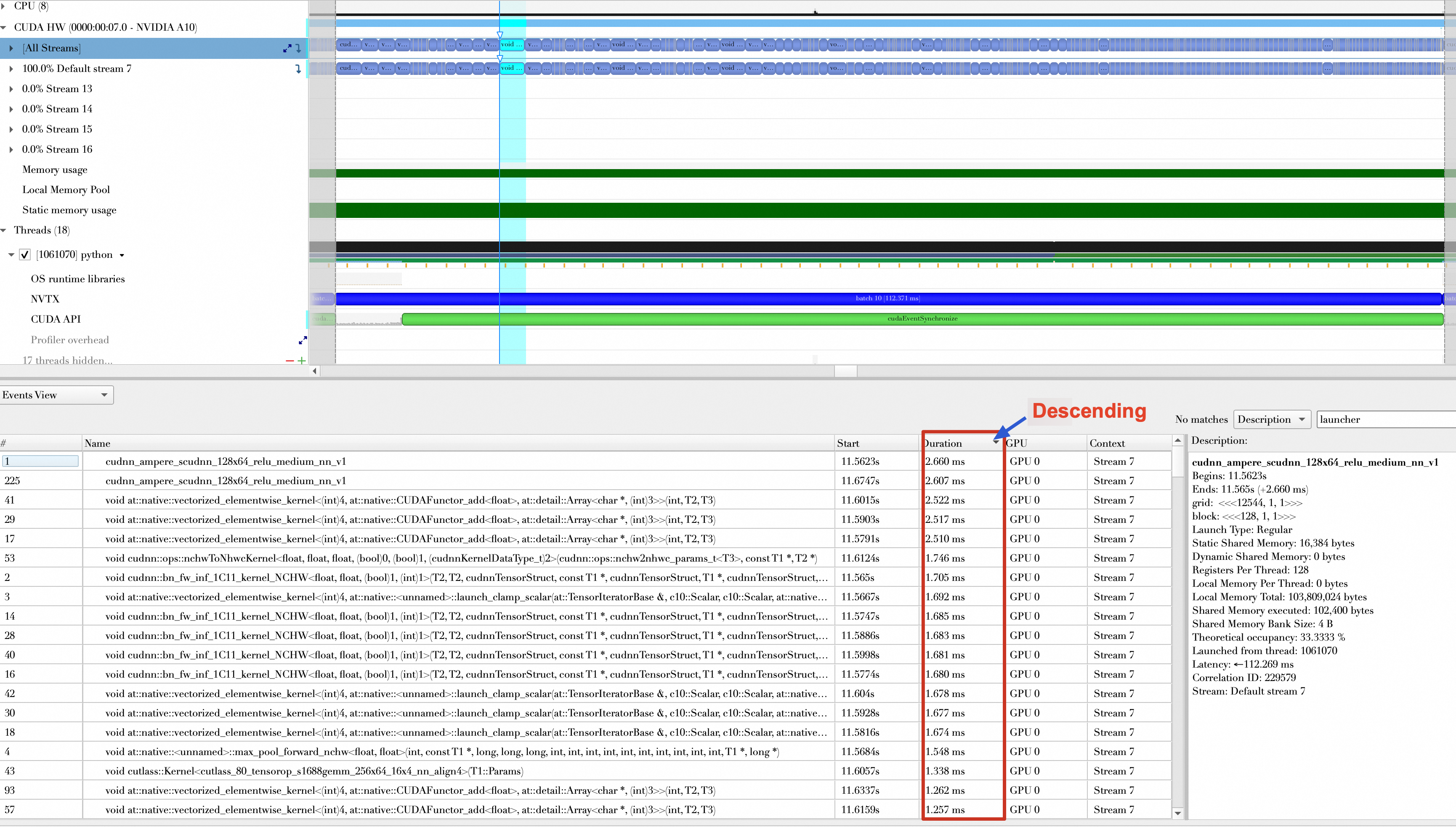
Data precision calibration (quantization)
Next, you can use the Nsight Systems UI to compare the results before and after quantization.
No model optimization | Optimize model with TensorRT without quantization | Optimize model with TensorRT and enable quantization |
|
|
|
Conclusion
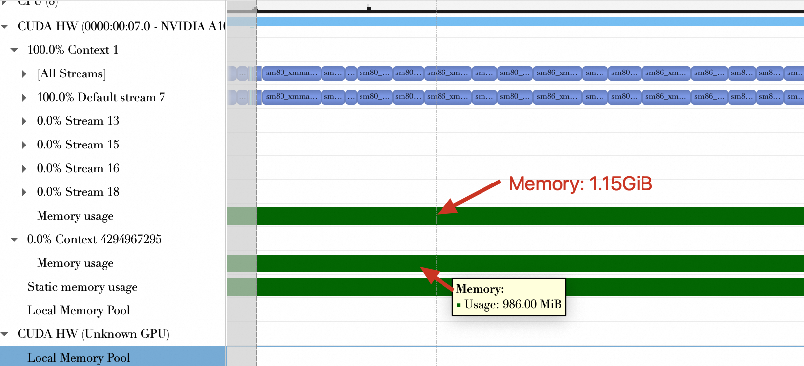
Comparison item | No model optimization | With TensorRT (quantization disabled) | With TensorRT (quantization enabled) |
Average time of top 15 longest-running functions (ms) | 1.98 ms | 1.51 ms | 772.76 μs |
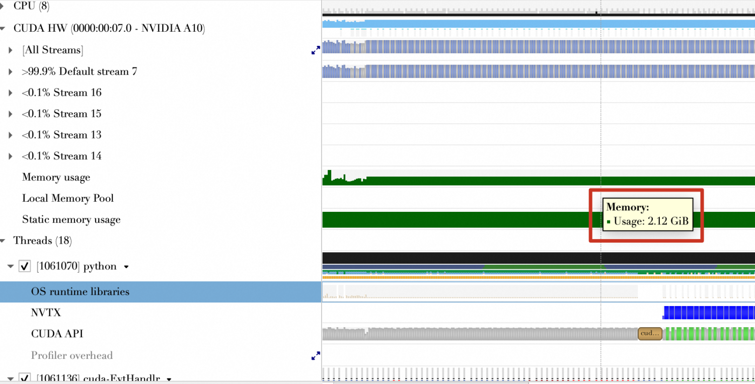
Memory usage (GiB) | 2.12 GiB | 2.13 GiB | 1.65 GiB |
Quantization reduces both kernel computation time and GPU memory usage.
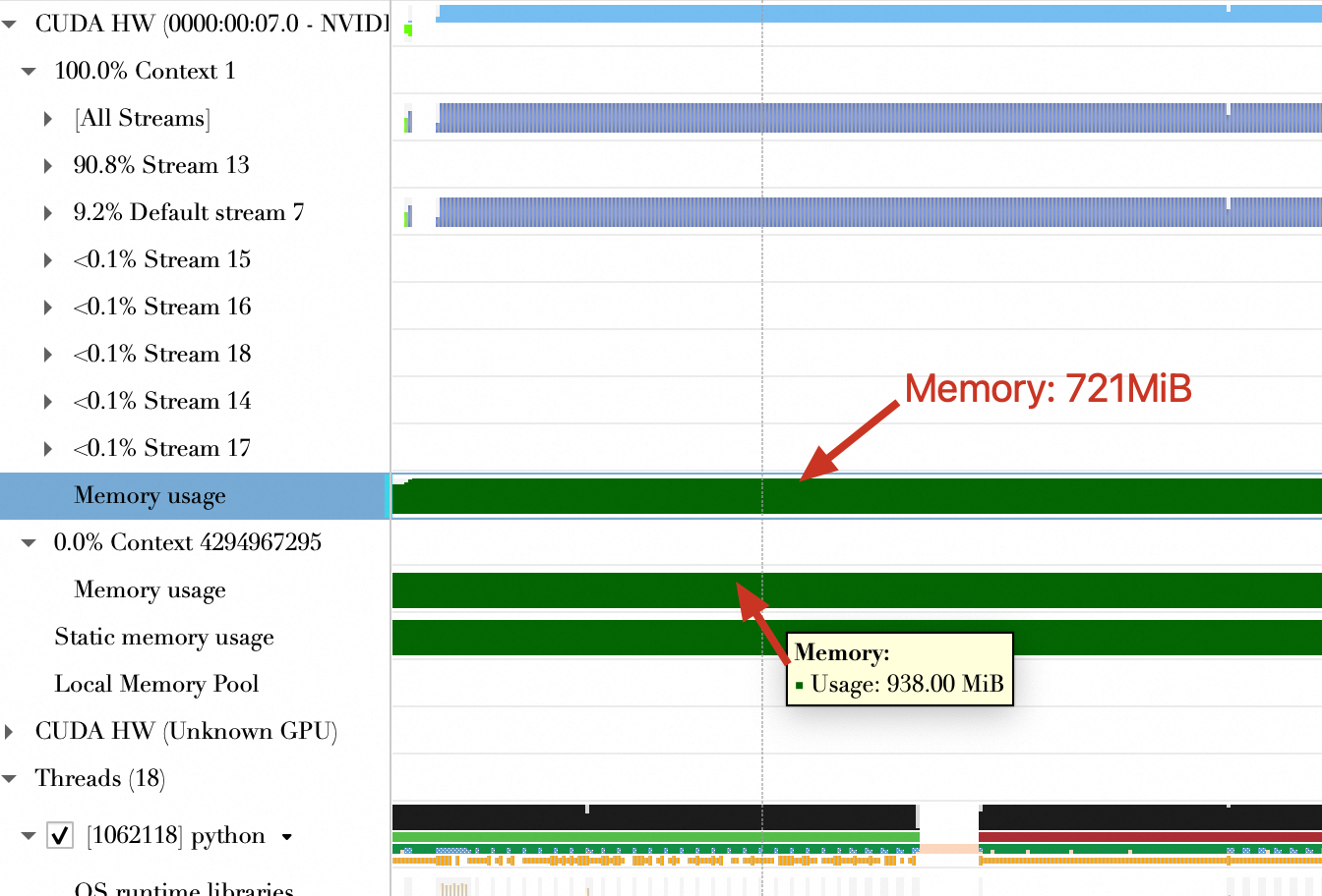
Dynamic Tensor Memory
No model optimization | Optimize model with TensorRT without quantization | Optimize model with TensorRT and enable quantization |
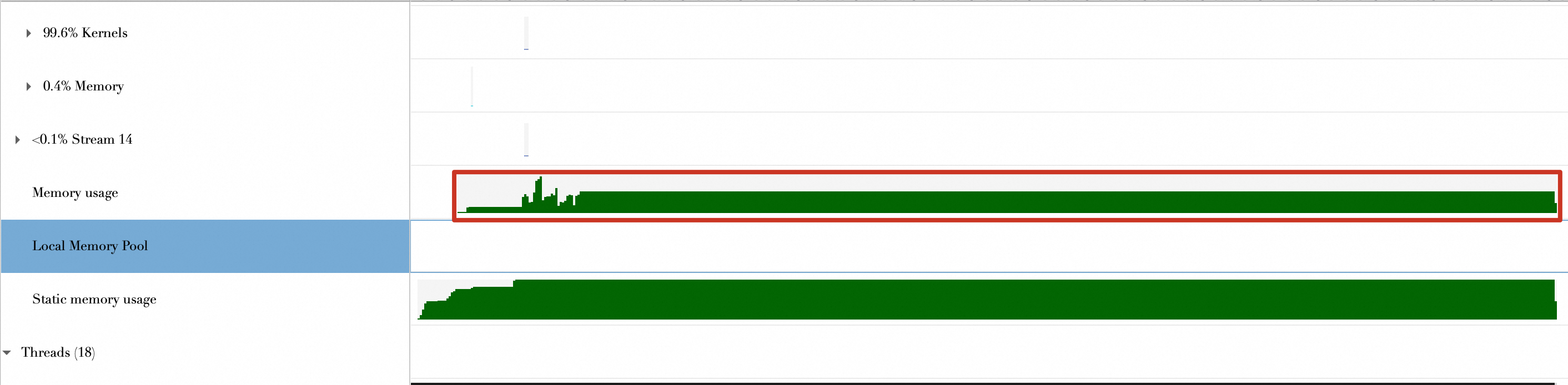
The memory usage throughout the program's lifecycle shows almost no change.
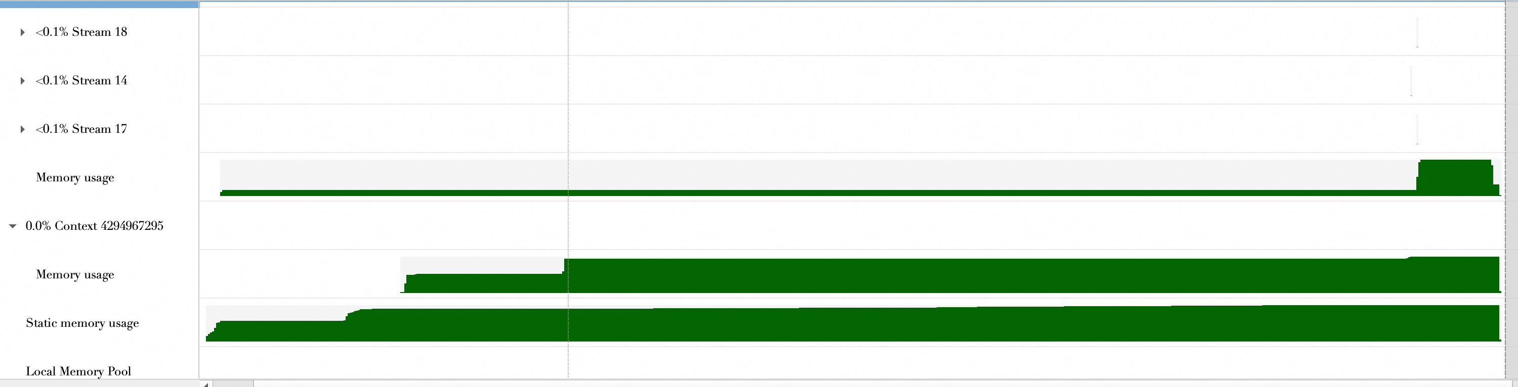
| The memory usage throughout the program's lifecycle shows a stepped pattern, which indicates dynamic on-demand allocation.
| - |
Multi-Stream Execution
No model optimization | Optimize model with TensorRT without quantization | Optimize model with TensorRT and enable quantization |
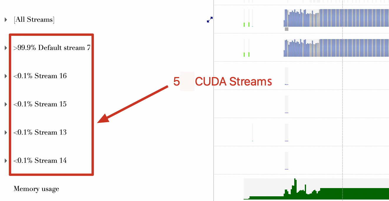
The figure below shows 5 CUDA streams.
| The figure below shows 5 CUDA streams.
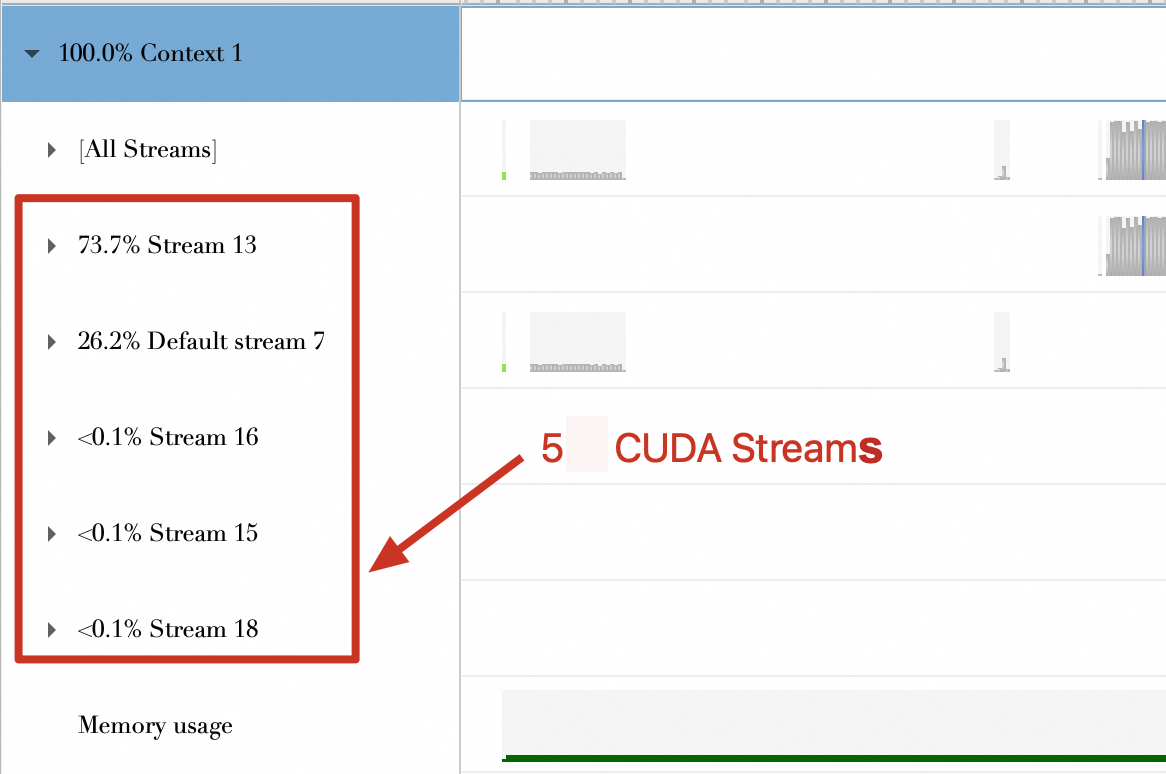
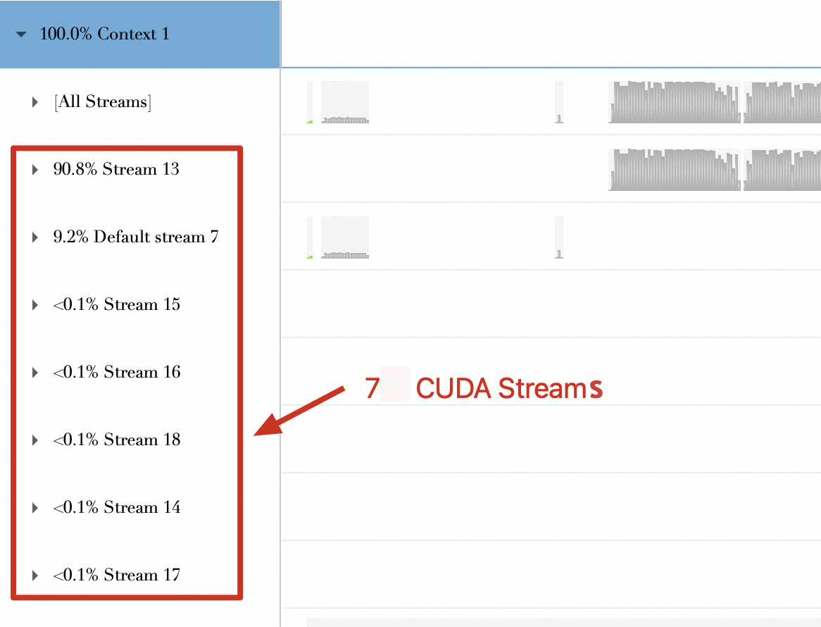
| The figure below shows 7 CUDA streams.
|
Conclusion
TensorRT supports dynamic multi-stream creation, but it is unclear whether this requires quantization to be enabled.
Migration scenarios
PyTorch and TensorFlow support environment awareness. Applications, such as inference services or training jobs, can be migrated from a CPU to a GPU without code changes. The application uses the GPU if it is available, or otherwise uses the CPU. However, in practice, migrated applications often run slowly.
This happens because the code was not designed to offload more computation to the GPU. After migration, the GPU utilization remains low while most of the computation remains CPU-bound, which leaves the GPU idle most of the time.
In migration scenarios, the best practice is to profile the application with Nsight Systems and Nsight Compute to find optimization opportunities, and then run the optimized application in the new environment.
FAQ
Question 1: Why use Pin Memory to reduce data transmission time?
By default, allocated host memory is pageable. Page fault operations, which are triggered by the OS, move data between physical locations in the host virtual memory.
GPUs cannot safely access pageable host memory because they cannot control when the host OS moves data. When you transfer data from pageable host memory to device memory, the CUDA driver first allocates temporary page-locked (pinned) memory, copies the data from pageable memory to pinned memory, and then transfers the data to the device memory. If you use pinned memory directly, you can skip the copy step from pageable to pinned memory, which saves time.
Question 2: How does batch loading overlap with batch computing?
First, it is important to understand CUDA streams. They work like first-in, first-out (FIFO) queues, but they handle sequences of CUDA operations, such as transferring data from host memory to GPU memory, triggering GPU kernel execution, or reverse data migration. Operations are executed strictly in the order that they enter the stream, which establishes clear timing.
Furthermore, the interaction between CUDA operations and CPU processes falls into two categories: synchronous and asynchronous.
Synchronous operations: These act as a "checkpoint" for the CPU process. When a synchronous operation is encountered, the CPU pauses until the operation is complete. The CPU places the operation at the end of the stream and temporarily blocks new entries until the operation is complete. Therefore, the duration of a synchronous operation varies with the pending tasks in the queue.
Asynchronous operations: The CPU adds the operation to the stream queue and immediately continues with other tasks without waiting. This avoids direct CPU waiting points.
Finally, it is important to note a key detail about PyTorch. By default, PyTorch automatically creates and uses one stream, the default stream, for all CUDA operations. This is essential for GPU-accelerated computing.