Continuous profiling
Continuous profiling helps you identify CPU, memory, and I/O bottlenecks in Java programs. It provides detailed statistics by method name, class name, and line number. This information helps developers optimize programs, reduce latency, increase throughput, and save costs. This topic describes how to enable the continuous profiling feature of Application Real-Time Monitoring Service (ARMS) and view the profiling data.
Performance tests show that for a typical Spring Web application with all features enabled, continuous profiling increases CPU overhead by about 5% and off-heap memory overhead by about 50 MB. The impact on garbage collection (GC) and request latency is minimal.
Prerequisites
Continuous profiling data is stored for only 7 days in Simple Log Service (SLS) under your account. The data is stored in the `proj-xtrace-<encode>-<region-id>` project and the `logstore-profiling` Logstore.
You have connected your application to CloudMonitor 2.0.
The continuous profiling feature currently supports only OpenJDK and Oracle JDK. It does not support IBM OpenJ9 or Oracle GraalVM JDK.
Limits
Operating system kernel
Linux 2.6.32-431.23.3.el6.x86_64 or later.
You can run the uname -r command to check the current kernel version.
JDK version
Continuous profiling uses the Java Virtual Machine Tool Interface (JVM TI) to retrieve the application's method stack. This provides details about CPU and memory usage while the application is running. JVM TI has a known crash issue that can cause applications to crash. This issue is fixed in OpenJDK 8u352, 11.0.17, and 17.0.5, and in Oracle JDK 11.0.21 and 17.0.9. For JDK versions released before this fix, the ARMS team ran multiple tests and found that the issue occurs only in specific scenarios and is very rare. Therefore, ARMS does not disable continuous profiling if your JDK version is not up to date. You can enable the feature temporarily and limit its scope by application IP address. However, to ensure application stability, upgrading your JDK is highly recommended. Using continuous profiling on older JDK versions poses a risk of application crashes.
Continuous profiling depends on debug symbols in the JDK. Alpine base images remove these symbols to reduce size, which prevents the feature from working correctly. To use continuous profiling, consider using a non-Alpine base image.
Recommended JDK versions for continuous profiling:
JDK Type | Version |
OpenJDK |
|
Oracle JDK |
|
Enable continuous profiling
Log on to the Cloud Monitor 2.0 console, and select a workspace. In the left navigation pane, choose .
On the Application List page, click the name of the target application. In the top navigation bar, choose .
In the Continuous Profiling Settings section, turn on the main switch and set the Real-time IP or Real-time CIDR block.
Click Save.
View continuous profiling data
Log on to the Cloud Monitor 2.0 console, and select a workspace. In the left navigation pane, choose .
In the top navigation bar, choose .
On the Application List page, click the target application. Then, in the top navigation bar, choose .
Query data

Filter metadata (① in the figure)
Profile metadata includes the application name and profile type. You can use these to identify a set of profiles.
When you select a set of metadata, the system automatically updates the trend graph and flame graph.
NoteChanging the selected metadata clears any existing tag filters in the Quick Filter area.

Set the time range for metadata (② in the figure)
This time range specifies the data retrieval scope for metadata and quick filters. The default is the last 15 minutes to ensure a fast response. You do not usually need to change this. Adjust the time range if data fluctuates frequently or has large gaps.
This setting affects only the time range for the trend graph and flame graph, not for the metadata. Auto-refresh is supported.
Quick filter (③ in the figure)
Quick filter data depends on the metadata time range. The tag keys are retrieved from the
labelsfield (in JSON format) of the performance monitoring data. The filters are combined using AND logic. When you select tags, the system automatically updates the trend graph and flame graph.Host Address: The IP address of the instance where profiling started.
Thread Name: All application threads. You can find abnormal threads based on CPU time consumption, memory usage, and other metrics.
Thread Group Name: Displays thread groups, which are collections of threads with the same rules. You can find categories of abnormal threads based on CPU time consumption, memory usage, and other metrics.
Trend graph (④ in the figure)
This graph shows the trend of the profile metadata within the specified time range.
Flame graph (⑤ in the figure).
After you select the metadata, tags, and time range, the system automatically generates a flame graph for the profile set.
Click the
 icon to view the problems and suggestions that Copilot provides for the current flame graph. You can also ask custom questions to learn more about CPU, memory, and flame graph data.
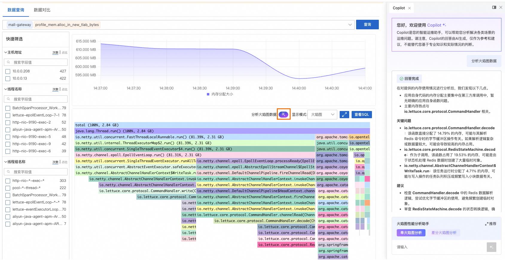
Set Display Mode to Flame Graph Only, Table Only, or Table + Flame Graph.
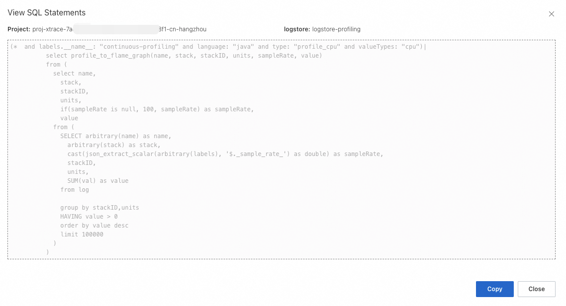
Click View SQL to view the SQL statement used to build the flame graph. You can use this statement to perform data analytics in the corresponding project and Logstore of SLS.
Compare data
Data comparison lets you compare the values of a target profile between a current time period and a past time period.
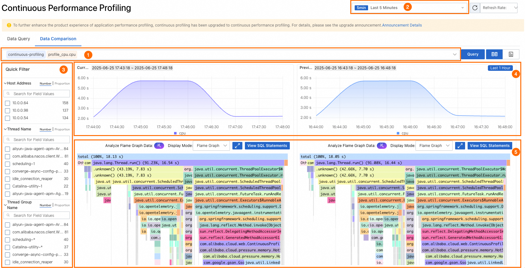
Filter metadata (① in the figure)
Profile metadata includes the application name and profile type. You can use these to identify a set of profiles.
When you select a set of metadata, the system automatically updates the trend graph and flame graph.
NoteChanging the selected metadata clears any existing tag filters in the Quick Filter area.

Set the time range for metadata (② in the figure)
This time range specifies the data retrieval scope for metadata and quick filters. The default is the last 15 minutes to ensure a fast response. You do not usually need to change this. Adjust the time range if data fluctuates frequently or has large gaps.
This setting affects only the time range for the trend graph and flame graph, not for the metadata. Auto-refresh is supported.
Quick filter (③ in the figure)
Quick filter data depends on the metadata time range. The tag keys are retrieved from the
labelsfield (in JSON format) of the performance monitoring data. The filters are combined using AND logic. When you select tags, the system automatically updates the trend graph and flame graph.Host Address: The IP address of the instance where profiling started.
Thread Name: All application threads. You can find abnormal threads based on CPU time consumption, memory usage, and other metrics.
Thread Group Name: Displays thread groups, which are collections of threads with the same rules. You can find categories of abnormal threads based on CPU time consumption, memory usage, and other metrics.
Trend graph (④ in the figure)
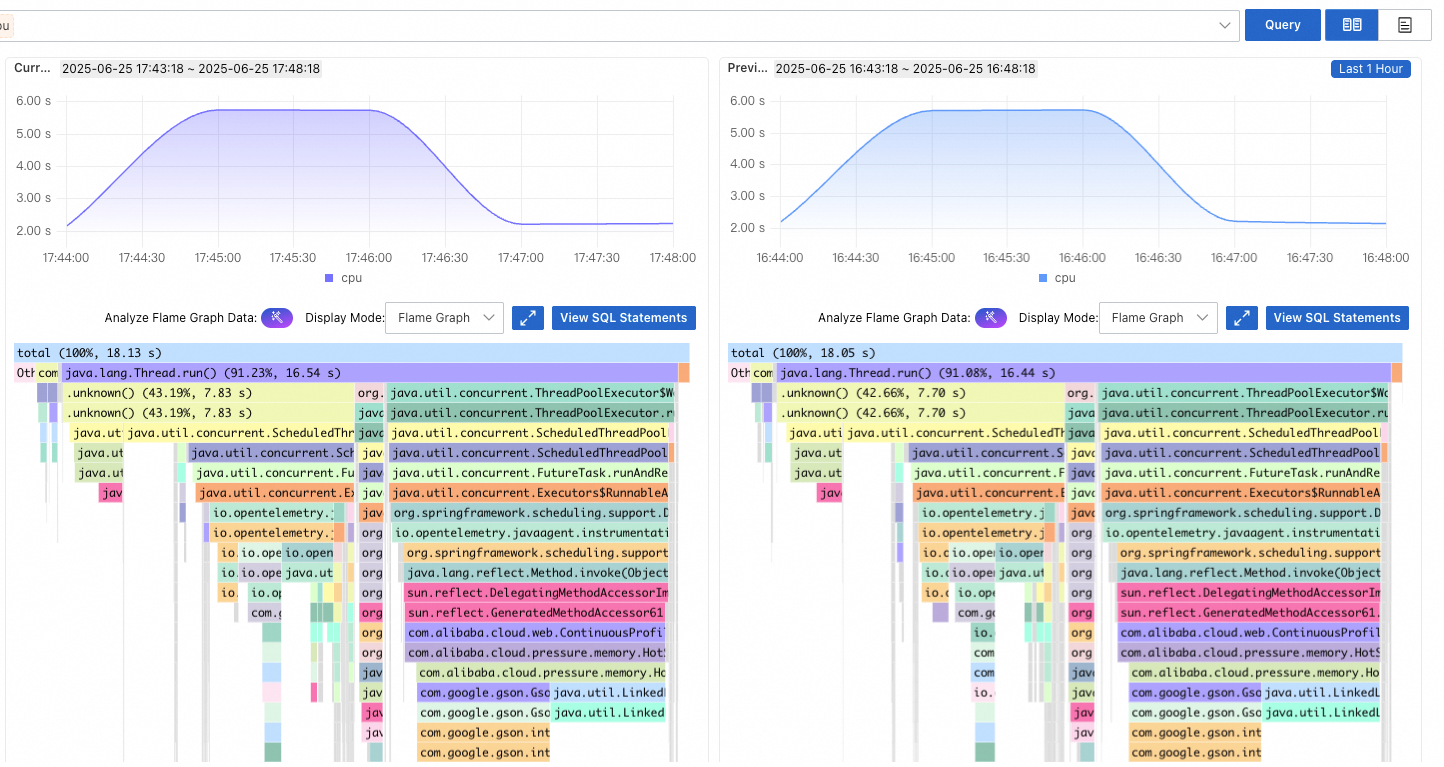
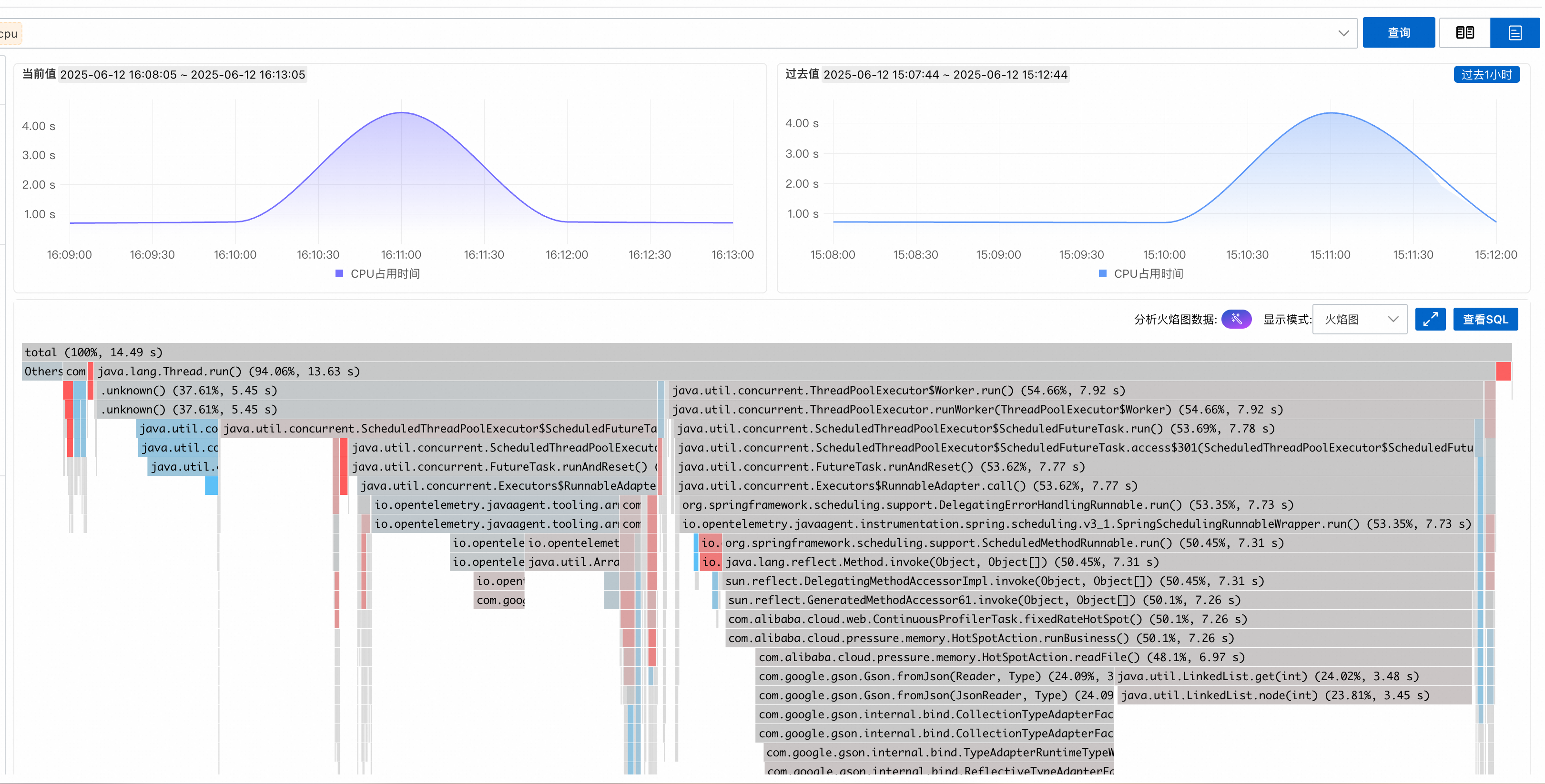
The trend graph shows data fluctuations and overall trends for a current period and a past period. The graph is based on filtered metadata and tags, aggregated over time. The aggregation policy is derived from the metadata section.
In the Current Value section, the time range is the same as the main time range (② in the figure). In the Past Value section, click Past N Hours to specify the comparison period.
Flame graph (⑤ in the figure).
After you select the metadata, tags, and time range, the system automatically generates a flame graph for the profile. Click the
icon to switch between the simple comparison view and the merged comparison view.Simple comparison view
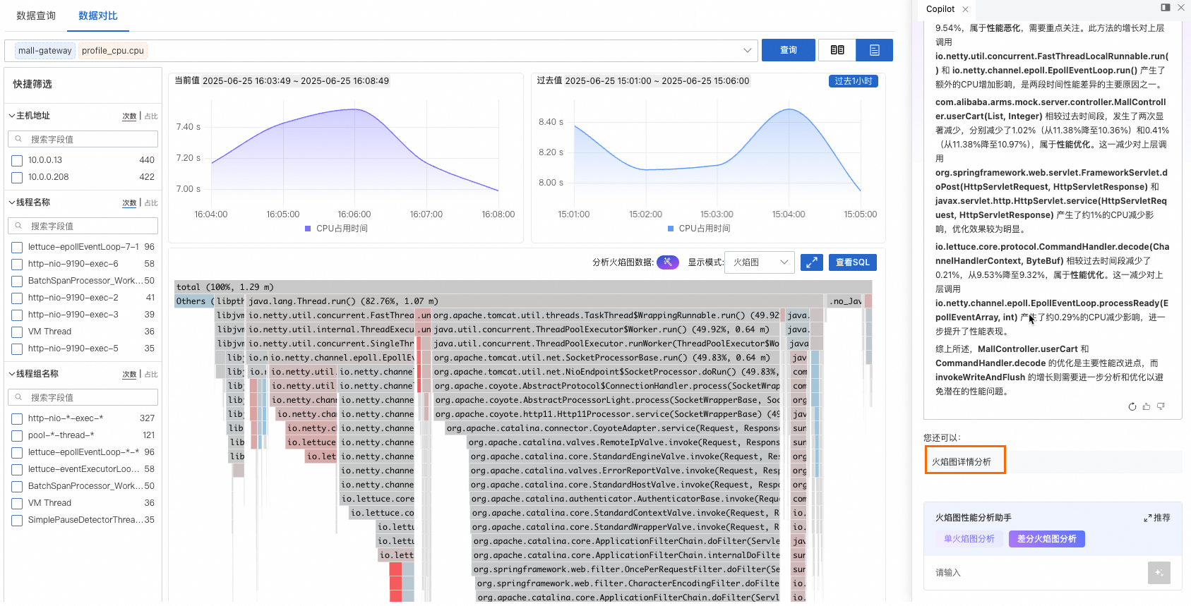
Merged comparison view
Red indicates an increase in proportion compared to the past. Blue indicates a decrease.
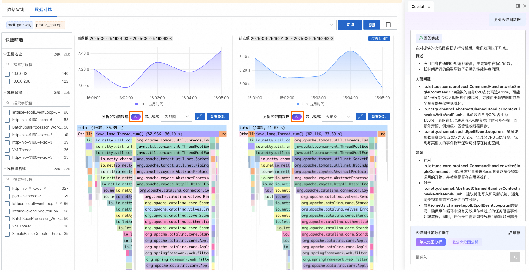
Click the
icon to view the problems and suggestions that Copilot provides for the current flame graph. You can also ask custom questions to learn more about CPU, memory, and flame graph data.In the merged comparison view, Copilot compares the profiling data from the two periods. It highlights performance changes and influencing factors. Click Flame Graph Details Analysis to have Copilot analyze specific performance issues and suggest fixes.
Set Display Mode to Flame Graph Only, Table Only, or Table + Flame Graph.
Click View SQL to view the SQL statement used to build the flame graph. You can use this statement to perform data analytics in the corresponding project and Logstore of SLS.

 icon to switch between the simple comparison view and the merged comparison view.