Viewing reports in Asight Systems GUI
The Asight Systems GUI displays collected reports. The following figure shows the GUI with a report open:
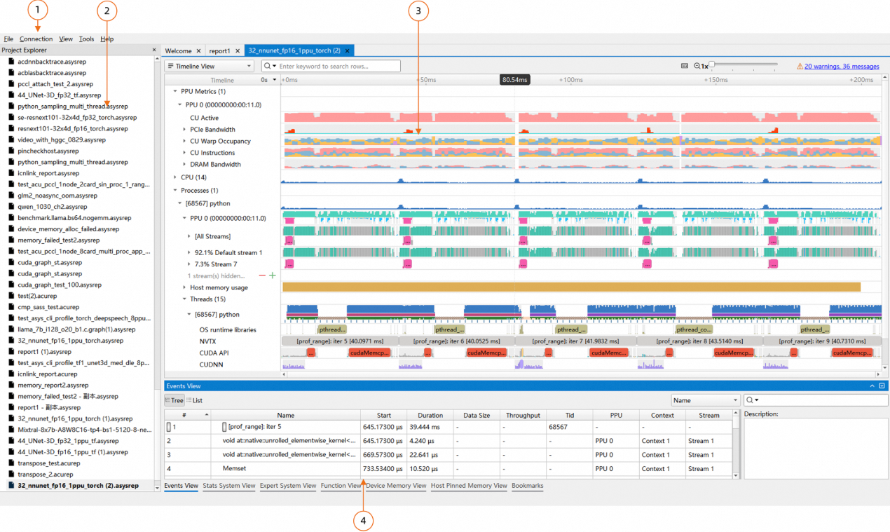
The main GUI components are:
Menu Bar. For details, see menu bar.
Project Explorer. For details, see Project Explorer.
Timeline View. For details, see Timeline View.
Events View. For details, see Events View.
1. Menu bar
The menu bar in the Asight Systems GUI is shown below:

File
Open: Opens a report.
Open Advanced: Opens a report using the advanced open feature. For details, see Advanced open feature for reports.
Exit: Exits the Asight Systems GUI.
Connection
Connect: Opens the Connection Dialog. For details, see Connection Dialog.
View
Show Project Explorer: Shows or hides the Project Explorer.
Show Output Messages: Shows or hides the Output Window.
Tools
Options: Opens the Options Dialog. For details, see Options.
Help
Documentation: Opens the Asight Systems user manual.
About: Displays information about Asight Systems.
1.1 Advanced open feature
Use the advanced open feature for reports to:
Open multiple reports in the same Timeline View.
Open a specific portion of a report based on percentage.
Specify which event types to load; only selected types are loaded when the report is opened.
To access this feature, select File > Open Advanced. The UI appears as follows:
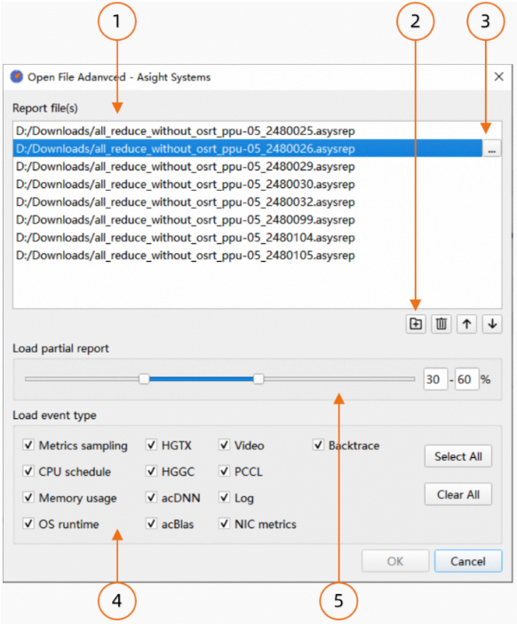
A list of the reports to open. These reports appear in the same Timeline View.
The control buttons for the report path list. From left to right, use these buttons to:
Add a new path.
Remove the selected path.
Move the selected path up one row.
Move the selected path down one row.
A button that opens a file browser to select a new path to replace the selected path.
A section for selecting event types. Only the checked event types are loaded.
A slider to select the portion of the report to open. For example, the figure shows the slider set to open the 30% to 60% segment.
When you open multiple reports in the same Timeline View, their timelines appear chronologically based on when the events occurred. To align the timelines of different reports, see Aligning timelines for multiple reports.
2. Project Explorer
The Asight Systems GUI includes the Project Explorer to help you manage open reports:
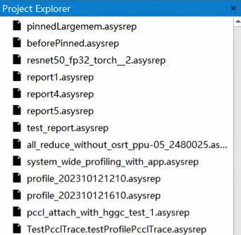
In the figure, a bold report name indicates that the report is open. The Project Explorer maintains a history of opened reports. You can remove an entry from the history by using its context menu. To quickly navigate to a report file's directory, right-click the report in the Project Explorer and select Show in Finder/Explorer from the context menu.
Tip: The Project Explorer only stores a reference to each report. If a report file is deleted or moved, this reference becomes invalid.
3. Timeline view
The Timeline View displays the timeline for all events, including HGGC, HGTX, OSRT, and CPU Sampling. Use the Timeline View to inspect PPU and CPU workloads and accurately pinpoint bottlenecks. The Timeline View is divided into two parts: the Timeline Area at the top and the Events View at the bottom, as shown in the following figure:
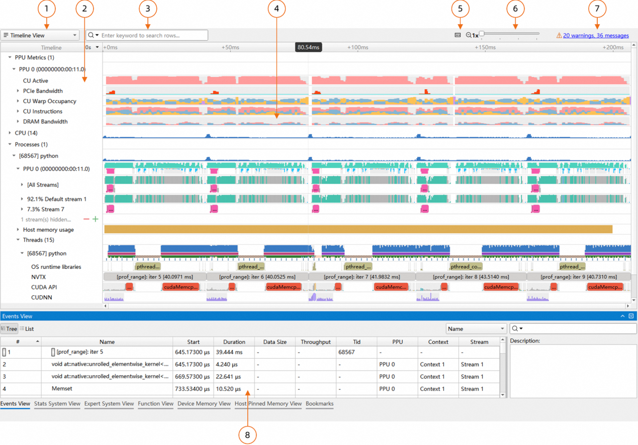
Page-switching drop-down list: Switches to the Analysis Summary View.
Timeline Tree
Search box
Timeline Area
Operation guide button: Opens the operation guide.
Vertical zoom slider: Zooms the timeline vertically.
Click to switch to the Diagnostics Summary View.
Events View
Collected events are organized in a tree structure in the Timeline Tree on the left. If a specific collection is disabled, its corresponding row is not displayed in the timeline.
3.1 Operation guide
The Asight Systems GUI supports various operations to navigate the timeline. The operation guide lists the supported actions and their shortcuts:
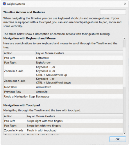
Keyboard and mouse operations
Action | Keyboard and mouse |
Pan left | ← or A |
Pan right | → or D |
Zoom in horizontally | + or = or W or Ctrl/Command + Scroll wheel up |
Zoom out horizontally | - or S or Ctrl/Command + Scroll wheel down |
Next row | ↓ |
Previous row | ↑ |
Undo | Backspace |
Trackpad operations
Action | Trackpad |
Pan left | Two-finger swipe left |
Pan right | Two-finger swipe right |
Zoom in horizontally | Two-finger pinch out |
Zoom out horizontally | Two-finger pinch in |
Scroll up | Two-finger swipe down |
Scroll down | Two-finger swipe up |
Selecting an item
Action | Keyboard and mouse |
Select an item in the timeline | Left-click |
Select an item in the Events View | Double-click |
Select an item and zoom to fit screen | Ctrl/Command + Left-click |
Selecting a time range
Action | Keyboard and mouse |
Select a time range | Left-click and drag |
Drag the selected time range | Left-click and drag |
Deselect the time range | Esc or click outside the selected range |
Zoom to time range | Z |
Zoom to time range and deselect | Shift + Z or double-click the time range |
Filter by the current time range | F |
Filter by the current time range and deselect | Shift + F |
Vertical zoom
In addition to horizontal zoom, the Timeline View provides a vertical zoom feature. You can use the zoom slider in the upper-right corner:

Click the magnifying glass icon  on the left to reset the zoom.
Pin row
The Timeline View lets you pin rows. You can use the context menu or the Ctrl/Command + P shortcut to pin rows of interest to the top or bottom of the screen for easy comparison:
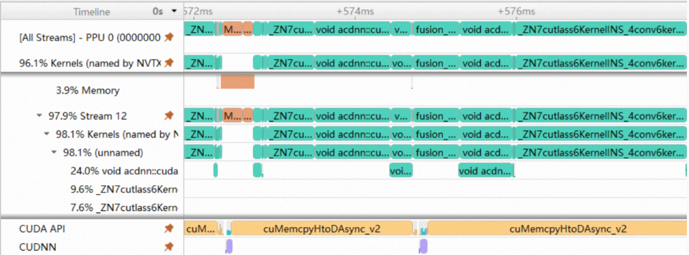
Hide trailing nodes
For a cleaner display, you can hide the trailing child nodes of certain nodes in the Timeline Tree:
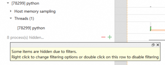
You can use the following operations to hide nodes:
Action | Keyboard and mouse |
Show one more node | Left-click "+" |
Show one fewer node | Left-click "-" |
Show five more nodes | Ctrl/Command + Left-click "+" |
Show five fewer nodes | Ctrl/Command + Left-click "-" |
Show all hidden nodes | Double-click |
You can also use the context menu for these operations:
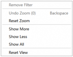
Action | Description |
Show More | Show one more node. |
Show Less | Show one fewer node. |
Show All | Show all nodes. |
Reset View | Restore the default display state. |
The node hiding feature is available for the following nodes:
CPU Core
Thread
Process
PPU Stream
PPU HGTX
PPU Kernel
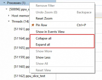
Expand/collapse all child nodes
For nodes with child nodes, you can use the context menu to expand or collapse all of them at once, as shown in the following figure:
Tooltip
All items in the Timeline View provide a tooltip. Hover over an item to view its details:
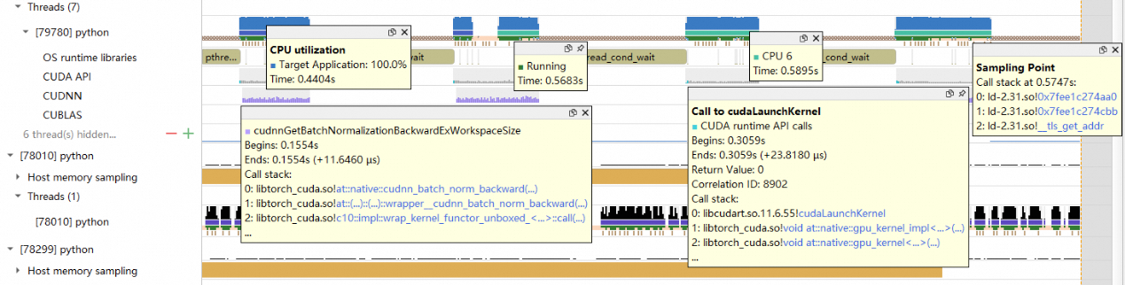
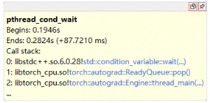
You can click the pin icon in the upper-right corner of the tooltip to keep it visible for easier reading. You can also click the copy icon to copy the tooltip's content.
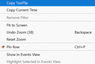
You can also export the tooltip content from the timeline by selecting context menu > Copy Tooltip:
Switch time axis display mode
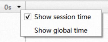
The time axis in the Timeline View has two display modes:
Session Time: This mode displays time with the report's start time as the origin (0) on the time axis, as shown in the following figure:

Global Time: This mode displays the actual wall-clock time.


You can switch between the two modes by clicking the triangle button on the left:
Dock widget
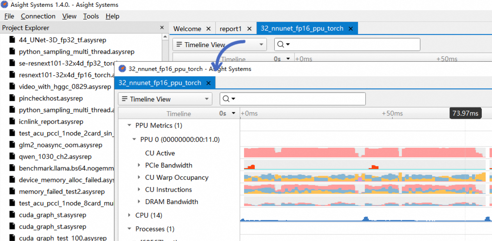
The UI supports dockable widgets, which you can drag out of the main window to view on a separate screen.
You can dock a widget by dragging its tab:
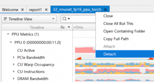
Alternatively, you can use the Detach/Attach options in the context menu:
Bookmark a timeline
The Timeline View allows you to bookmark timelines, making it easy to mark points of interest in large reports. You can add or remove a bookmark from the timeline's context menu:
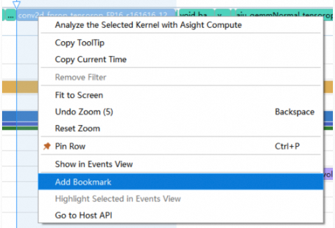
Creating a bookmark adds a persistent, numbered marker to the timeline:
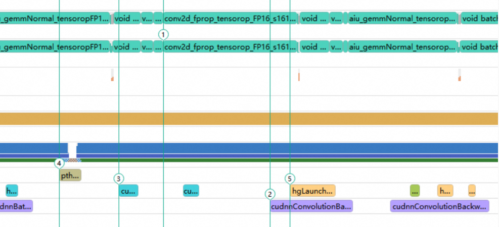
You can manage all your bookmarks in the Bookmarks window at the bottom:
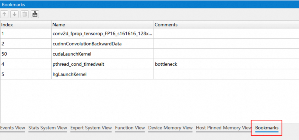
In this window, you can:
Change the bookmark number.
Add a note to a bookmark.
Clear all bookmarks at once.
Double-click an entry in the Name column or use the context menu to navigate to the corresponding timeline location.
3.2 Timeline item display strategy

The top of the Timeline View features a time axis where time progresses from left to right. For better readability, when you zoom in to a certain level, the Timeline View displays time in a baseline + increment format.
In the Timeline View, event timelines are called timeline items. Different types of timeline items are represented by different colors. An item's left edge marks the event's start time, its right edge marks the end time, and its width represents the event's duration.
When the Timeline View is not fully zoomed in, Asight displays events using an occupancy bar chart:
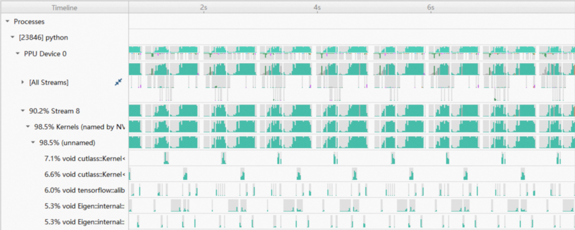
The figure above shows the kernel timeline as a series of bar charts with varying heights. This display strategy applies to various data types, including CPU utilization, thread and process occupancy, kernels, and Memcpy events.
Hierarchical operator display
In the Timeline View, communication operators are displayed in layers with distinct colors, for example, in the [All Streams] row:
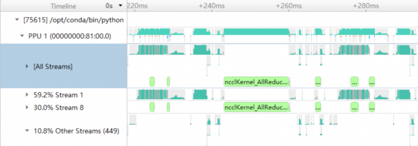
Color-coding kernels
To help distinguish between different kernel timelines, the Timeline View can display each kernel in a different color, as shown in the following figure:

You can enable this feature by navigating to Options Dialog > Systems Profile > Color HGGC Kernels.
3.3 Timeline correlation
When you select an item, the view highlights all related items:
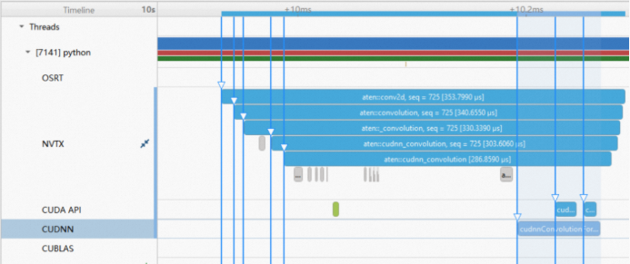
Events are correlated in the following two scenarios:
They belong to the same call stack, for example, an HGGC event nested within an HGTX event.
A host API call triggers a device activity, for example, a launch kernel API and its corresponding kernel.
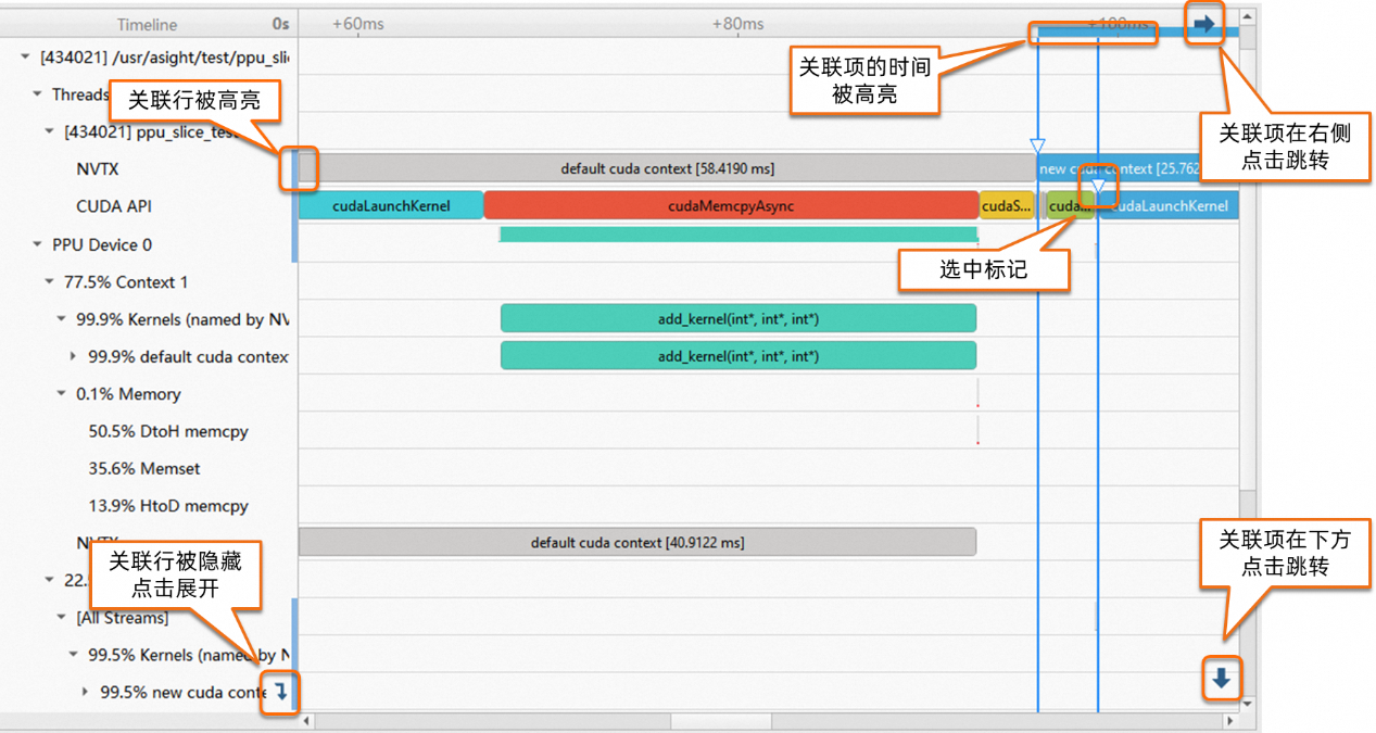
3.3.1 Correlation operations and markers
When an item is selected, corresponding markers and buttons appear in the Timeline View:
3.4 Selecting a time range
The Timeline View allows you to select a time range by clicking and dragging with the left mouse button, as shown in the following figure:
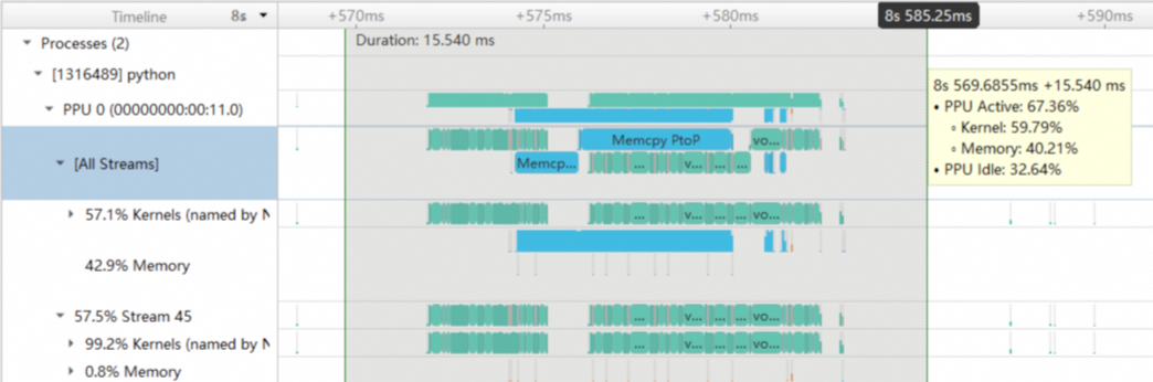
When you select a time range, a tooltip appears, showing the start time and duration of the range. It also displays the percentage of PPU active/idle time, as well as the time spent on kernel execution and memory operations within the selected range.
When selecting or resizing a time range, you can hold down the Shift key to enable a snapping feature, which automatically snaps the range to the start or end point of the nearest timeline.
After selecting a time range, you can drag to change its position or resize it. Double-click the time range to zoom it to fit the entire screen. Asight Systems also supports filtering. You can use the context menu > Filter and Zoom in to isolate events within the current time range for further examination in the Events View.
3.5 Aligning timelines across reports
When you open multiple reports in the Timeline View, their timelines are displayed based on when the events occurred. To adjust the time offset between different reports, Asight Systems provides a timeline alignment feature, which can be accessed as shown below:
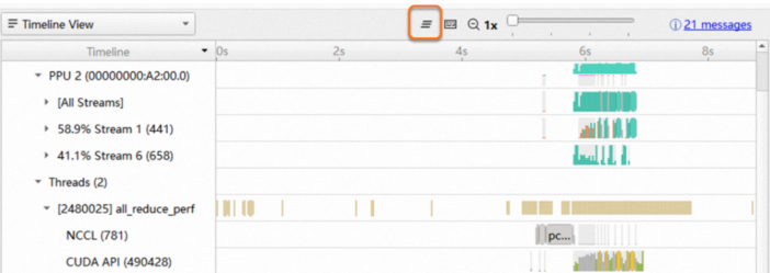
Clicking this opens the timeline alignment dialog:
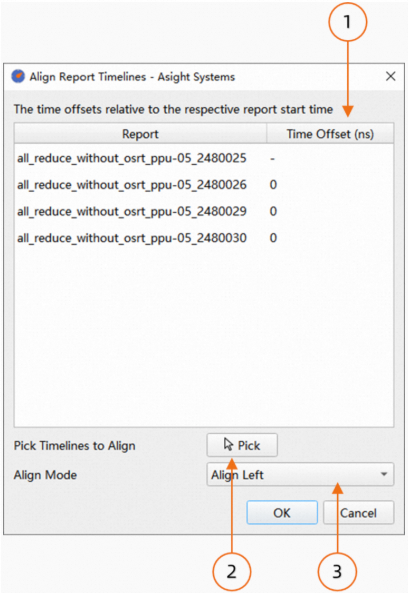
The time offset of each report's timeline relative to its collection start time, in nanoseconds. The default is 0. You can manually enter an offset for calibration.
Enter timeline picking mode to select a baseline timeline in each report for alignment.
Select the timeline alignment mode.
The Timeline View supports two alignment modes:
3.5.1 Manual alignment
If you know the time offset between reports, you can enter it manually in nanoseconds. A positive value shifts the timeline to the right; a negative value shifts it to the left. The offset for the first report in the list cannot be specified.
3.5.2 Semi-automatic alignment
If you know which events in the reports occurred simultaneously, you can use these timelines as a baseline for semi-automatic alignment. The Timeline View automatically calculates the time offsets between the reports based on these timelines.
First, click the Pick button to enter timeline picking mode:
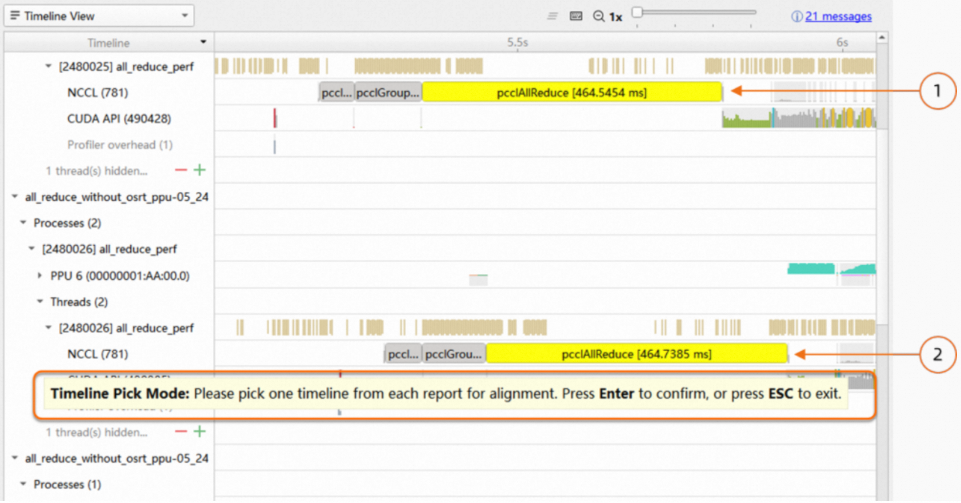
After entering this mode, the timeline alignment dialog disappears, and a tooltip appears at the bottom of the window. In the Timeline View, left-click to select the baseline timelines. The selected timelines are highlighted. You can only select one timeline per report; if you select another timeline in the same report, the previous selection is deselected.
After selecting the timelines, you can choose left-align or right-align in the timeline alignment dialog:
Left-align: The selected timelines started at the same time, aligning them by their left edges.
Right-align: The selected timelines ended at the same time, aligning them by their right edges.
You can exit timeline picking mode using the following keyboard actions:
Enter key: Confirms the selected timelines and reopens the timeline alignment dialog.
Esc key: Discards the selection and reopens the timeline alignment dialog.
If you confirm the selected timelines, the timeline alignment dialog reappears as follows:
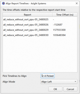
The dialog automatically calculates and populates the time offset for each report. The Pick button shows that four timelines have been selected. In the drop-down list below, you can select left or right alignment, and the time offsets above will be recalculated accordingly.
Tip: When picking baseline timelines, the time offsets are calculated relative to the timeline selected in the first report. If no timeline is selected for the first report, the offset is calculated from the start time of the first report in left-align mode, and from its end time in right-align mode. Therefore, it is recommended to always select a baseline timeline for the first report.
You do not have to select a timeline for every report. Reports without a selected timeline will not be aligned.
3.6 Searching and filtering rows
The search and filter feature for timeline rows helps you quickly find specific rows, as shown in the following figure:
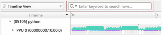
You can switch between two modes:
Search mode: Highlights matching items and allows you to navigate to the previous or next match.
Filter mode: Displays only the matching items.
The search results in search mode are shown in the following figure:
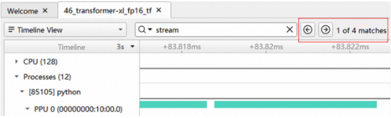
3.7 Using the Group View
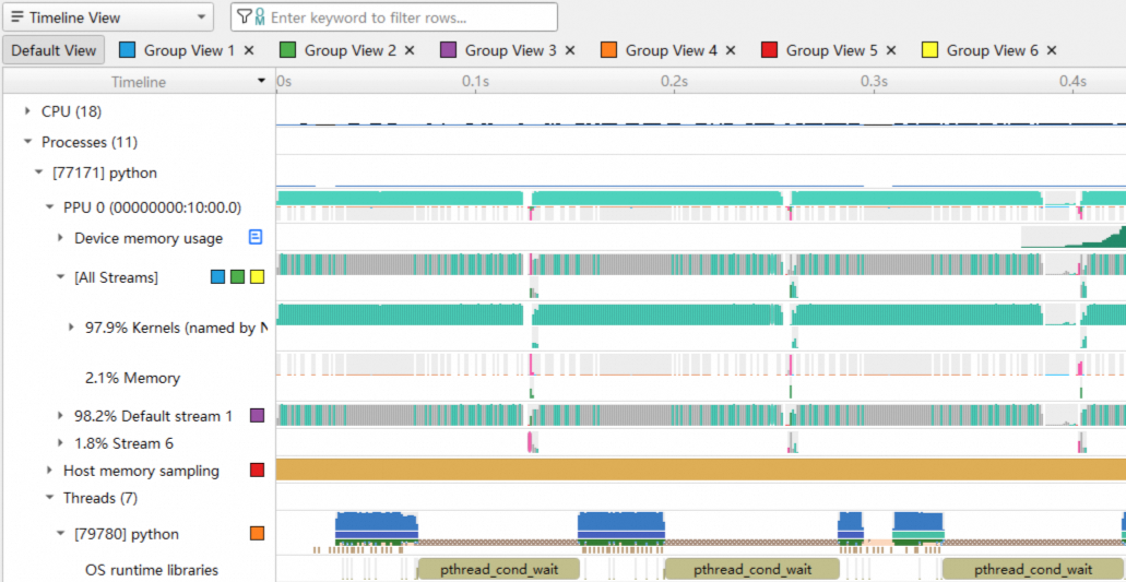
Large reports often contain a vast number of timelines. To make it easier to analyze specific timelines of interest, the Timeline View provides a grouping feature that allows you to add timelines to a Group View for isolated display.
You can right-click a timeline row of interest and add it to a Group View:
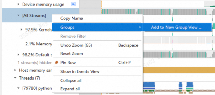
Once added, a button to switch to the Group View appears at the top of the Timeline View. A group icon also appears to the right of the timeline row, with its color matching the Group View button. Clicking this button switches to that Group View, as shown below:
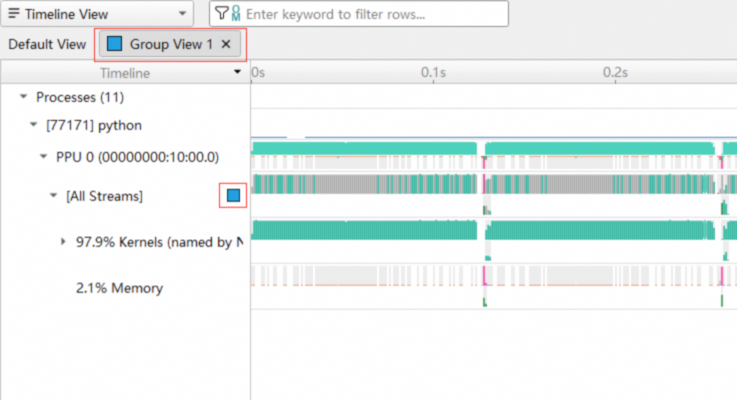
As you can see, only the [All Streams] row appears, while other related timeline rows are hidden. The following are also displayed along with the target row:
All ancestors of the target row
Child nodes of the target row
You can right-click the group button to rename the group:
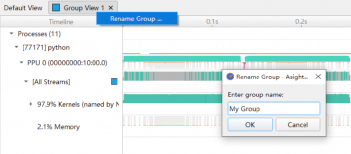
The same timeline row can be added to multiple Group Views:
3.8 Events View
The Events View displays events in a list format, supporting sorting, searching, and filtering of events, as well as navigation between the Events View and the Timeline View.
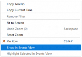
In the Timeline View, to display a node's events in the Events View, select Show in Events View from the context menu (shortcut: Shift + double-click):
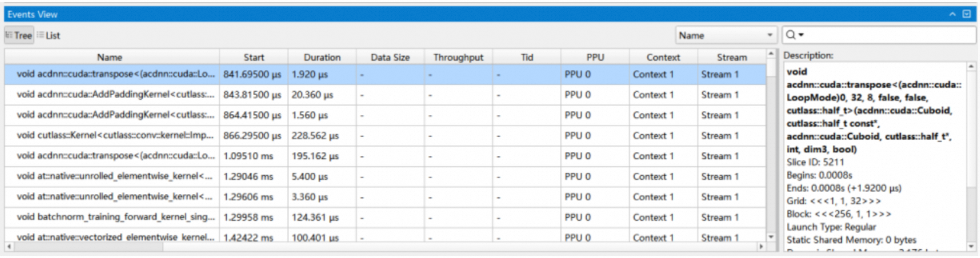
The Events View also displays the events of the selected node's children:
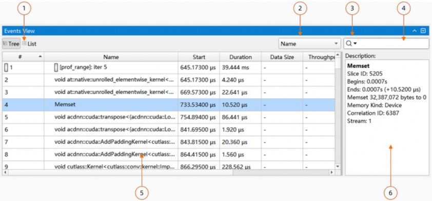
Select a display mode. For nested HGTX events, you can choose to display them in a tree or flat list format.
Select whether to search by Name or Description.
Advanced search options
Search bar
Events table
Description of the selected item, which is identical to the item's tooltip.
The table displays the following columns:
# (Index)
Name
Start
Duration
TID
If the Events View displays PPU-related nodes, it will also show the PPU, Context, and Stream columns:
After selecting events in the table, you can export the selection by choosing Copy from the context menu. You can select multiple items using Shift or Ctrl, or select all items by choosing Select All. To export all events directly to a CSV file, use Export All to CSV. You can sort the data in ascending or descending order by clicking the column headers.
3.8.1 Search
The Events View supports a search function:

It supports two search types:
Search by Name
Search by Description
It supports two modes:
Search
Filter
The search results are displayed as follows:
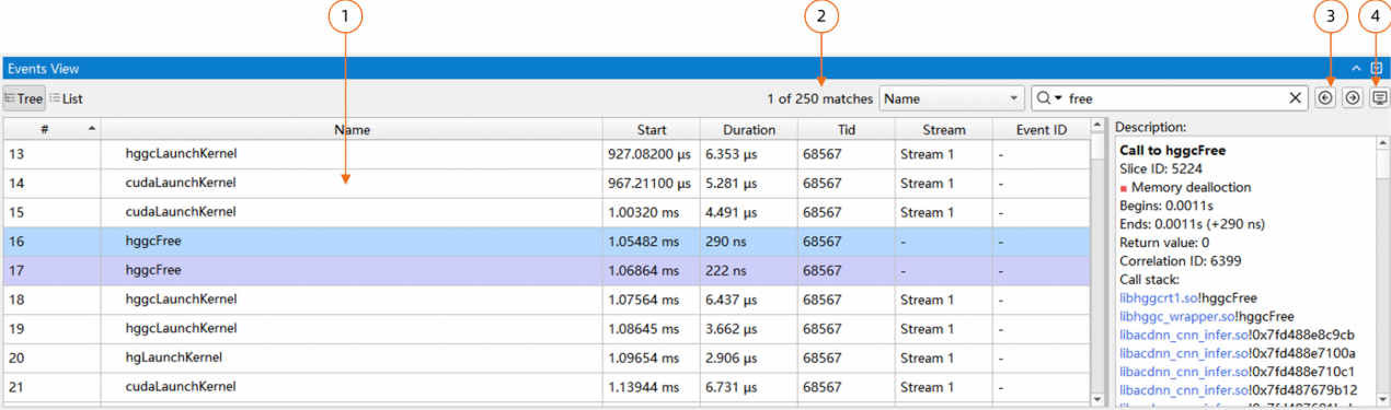
Search results are highlighted.
The number of matching items is displayed.
Navigation buttons allow you to jump to the previous or next match.
Search results are highlighted in the Timeline View.
The search bar and results are reset when you use Show in Events View again.
The Events View also supports advanced search options. Click the triangle button next to the magnifying glass to access them:
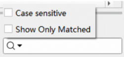
Case Sensitive: Determines if the keyword search is case-sensitive.
Show Only Matched: If checked, the Events View will only display matching items, hiding non-matching ones.
3.8.2 Navigating to the timeline
The Events View supports navigation to and from the Timeline View:
When a timeline item is displayed in the Events View, double-clicking the item in the timeline selects that item in the Events View.
Double-clicking an item in the Events View highlights the corresponding item in the timeline.
You can also navigate using the context menu:
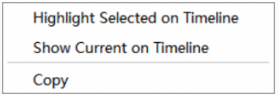
Highlight Selected on Timeline: Highlights the item in the timeline, which is the same as double-clicking the item.
Show Current on Timeline: Highlights the item in the timeline and zooms it to fit the entire screen.
3.8.3 Filtering by time range
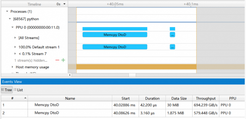
You can use the Events View to display only the events within a selected time range. First, select a time range in the timeline, then use the context menu to select Filter and Zoom in. The Events View will then only show events within that time range:
3.9 Function View
Asight Systems provides the Function View to analyze the CPU usage of all functions. The Function View presents CPU usage data in Top-Down, Bottom-Up, and Flat tables, as well as in flame graph and icicle graph formats. It supports sorting, searching, and filtering to help you quickly identify hotspot functions. To use the Function View, you must enable backtrace sampling during report collection. See Collect API Call Stacks.
3.9.1 Flame and icicle graphs
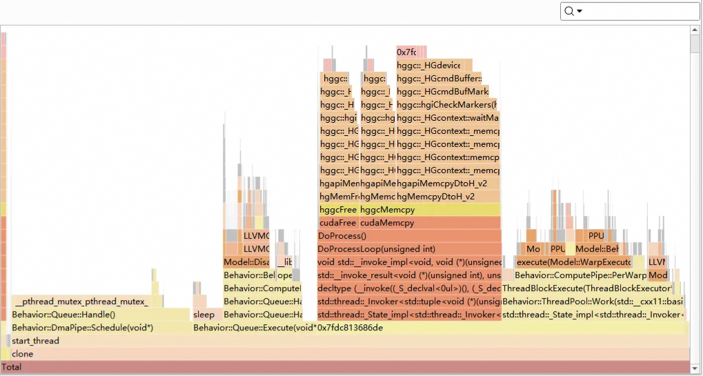
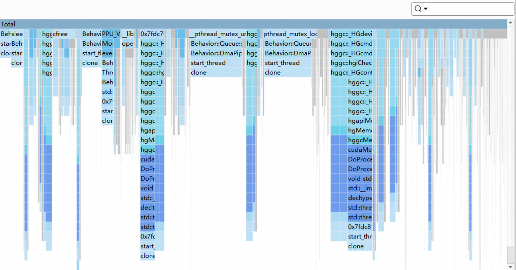
A flame graph helps you quickly find the call stack that consumes the most CPU time, while an icicle graph helps you quickly locate the function with the highest CPU consumption and its callers. Both graphs provide a high-level overview of the time consumed by all functions and help you quickly identify hotspot functions and their corresponding call stacks.
A flame graph is shown below:
An icicle graph is shown below:
Key features of flame and icicle graphs:
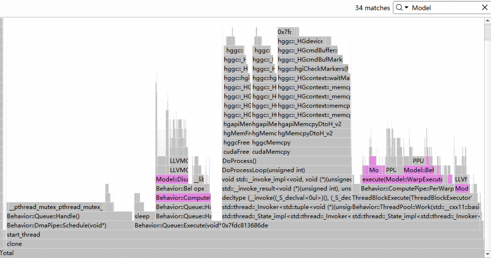
Each rectangle in the graph represents a function. The width of the rectangle indicates the CPU time consumed by the function, and the color distinguishes different modules. The x-axis does not represent the chronological order of functions. The y-axis represents the depth of the call stack, with callers at the bottom and callees at the top.
Hover over a function to see detailed CPU consumption, the function's module name, and other information in a tooltip or at the top of the graph.
Click a function to zoom in and view its detailed callers and callees.
Use the context menu on a function to copy its function name or module name.
You can search for functions. Search results are highlighted in magenta in the graph.
3.9.2 Function tables
Function tables include Top-Down, Bottom-Up, and Flat views. The main features are distributed as shown in the figure below:
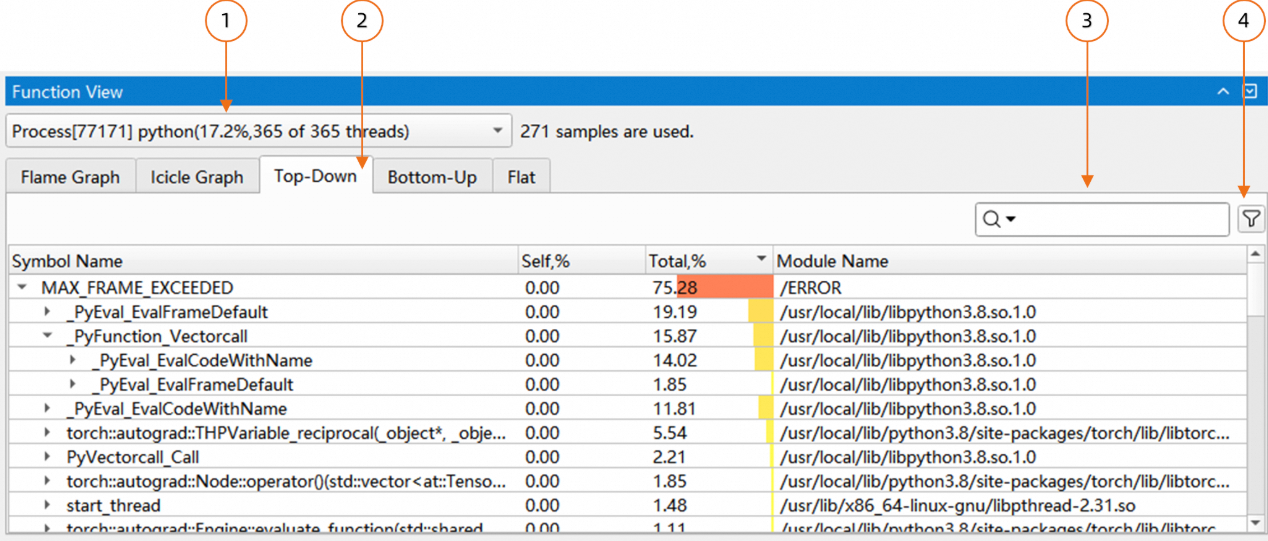
Select the target process to analyze.
Tab bar for switching to other sub-pages.
Search box
Filter Dialog
The Function tables display the following information:
Symbol name: The name of the function.
Self: The percentage of time consumed by the function itself.
Total: The percentage of time consumed by the function and the functions it calls.
Module name: The name of the module to which the function belongs.
The Function tables support sorting. Click a column header to sort the data in ascending or descending order.
The Function tables support searching for both Symbol Name and Module Name, with a Case Sensitive option. The search results are similar to those in the Events View and include:
Highlighted search results.
The number of matching items.
Navigation buttons to jump to the previous or next match.
The Function tables support filtering, including:
Hiding functions with a time percentage below a specified threshold (not hidden by default).
Specifying the number of decimal places for the time percentage.
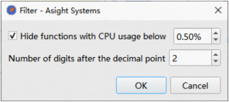
The Function tables support the following context menu functions:
Expand: Expands the selected row and all its child rows.
Collapse: Collapses the selected row and all its child rows.
Expand All: Expands all rows and their child rows in the table.
Collapse All: Collapses all rows and their child rows in the table.
Copy: Copies the content of the selected function to the clipboard.
Export All to CSV: Exports all functions in the table (including hidden rows) to a CSV file.
Top-Down Table
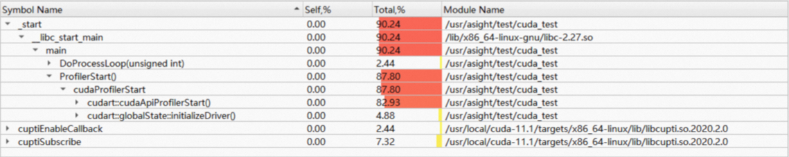
Taking the top-down mode of function time consumption as an example, the Top-Down view displays functions in a tree structure from the top-level callers to the bottom-level callees based on their call relationships. In the figure above, the main function calls both the DoProcessLoop and ProfilerStart functions, so they are both under the main node.
The main function has a Self value of 0, indicating that the logic within the main function itself is very simple. The Total value is 90.24%, indicating that the majority of the time is spent in the functions called by main.
Tip: The depth of the call stack is determined by the maximum stack unwinding depth specified during collection. If a function's call depth exceeds this maximum, the function at the top of the unwind at that point is treated as the root node.
If the name of a symbol cannot be obtained, the function's address is displayed instead.
Bottom-Up Table
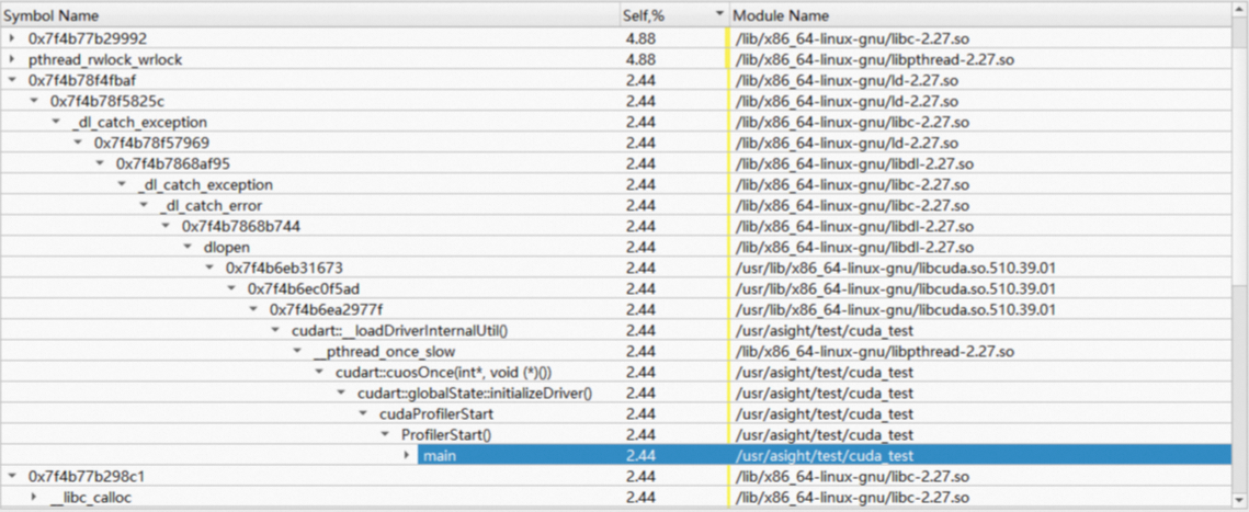
Taking the bottom-up mode of function time consumption as an example, the Bottom-Up view is the reverse of the Top-Down view. It starts with the function deepest in the call stack as the root node and the shallowest called function as the leaf node. For example, in the figure above, the main function is a leaf node. The Bottom-Up view does not display the Total column.
Flat Table
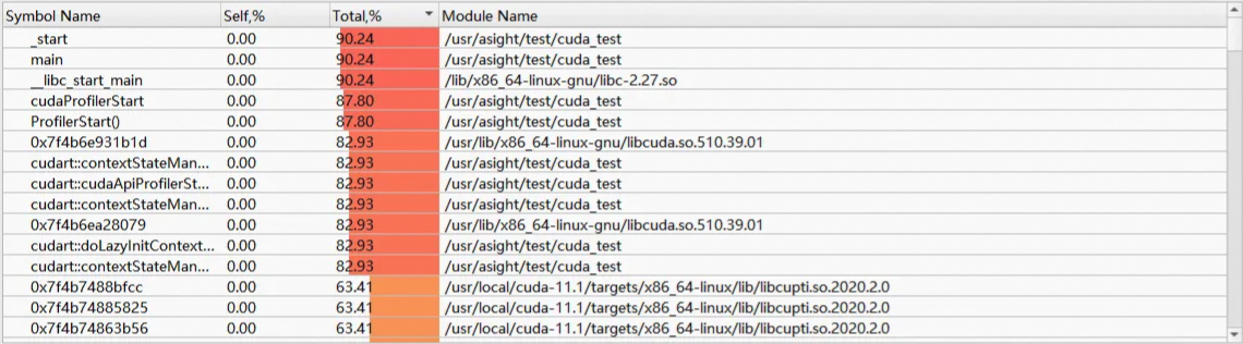
Taking the flat mode of function time consumption as an example, the Flat view displays all functions in a flat list. In scenarios where call relationships are not important, this view allows you to quickly find the functions with the highest Self and Total time consumption.
3.10 Device Memory View
Asight Systems provides the Device Memory View to analyze the device memory allocation and deallocation of all functions.
The Device Memory View supports four viewing modes, which can be switched from the drop-down list:

Unreleased Malloc Size: View the size of memory that was allocated but not released by each function.
Total Malloc Size: View the total size of memory allocated by each function.
Unreleased Malloc Count: View the number of memory allocations that were not released by each function.
Total Malloc Count: View the total number of memory allocations by each function.
The Device Memory View also supports flame graphs, icicle graphs, and Top-Down, Bottom-Up, and Flat tables. It includes sorting, searching, and filtering features to help you quickly identify hotspot functions. To use the Device Memory View, you need to enable device memory sampling as needed during report collection. See Analyze PPU Memory Usage.
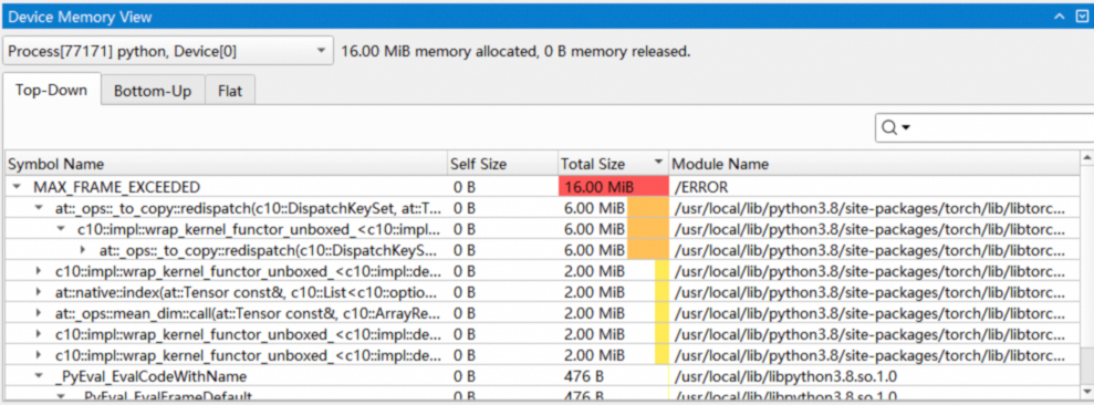
The table displays the following information:
Symbol name: The name of the function.
Self: The size of device memory allocated or deallocated by the function itself (positive values are allocations and are shown in red; negative values are deallocations and are shown in blue).
Total: The total size of device memory allocated or deallocated by the function and the functions it calls.
Module name: The name of the module to which the function belongs.
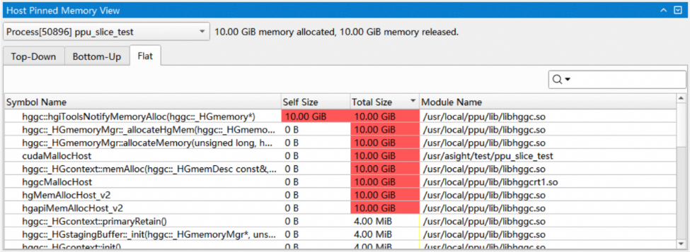
3.11 Host Pinned Memory View
Asight Systems provides the Host Pinned Memory View to analyze the pinned memory allocated and deallocated by all functions. Like the Device Memory View, it supports four viewing modes, flame graphs, icicle graphs, and Top-Down, Bottom-Up, and Flat tables. It also includes sorting, searching, and filtering features to help you quickly identify hotspot functions. To use the Host Pinned Memory View, you need to enable pinned memory sampling as needed during report collection. See Analyze Pinned Memory Usage.
3.12 Heap Memory View
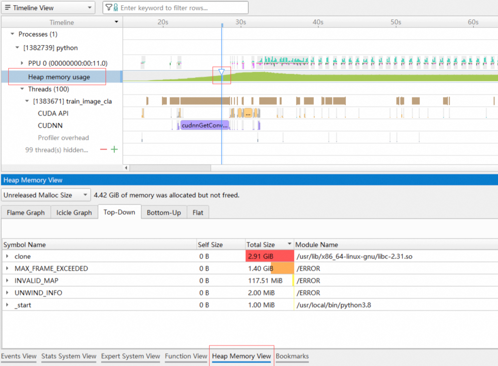
Asight Systems provides the Heap Memory View to analyze CPU-side dynamically allocated memory (heap memory) usage by functions. Like the Device Memory View, it supports four viewing modes, flame graphs, icicle graphs, and Top-Down, Bottom-Up, and Flat tables. It also includes sorting, searching, and filtering features to help you quickly identify hotspot functions. To use the Heap Memory View, you need to enable heap memory sampling as needed during report collection. See Heap Memory Usage Tracking. Click a time block in the Heap memory usage row of the Timeline View to see the process's memory usage information up to that point in time.
4. Analysis summary
The Analysis Summary page summarizes the report in multiple tables and shows the collection settings used to generate the report. You can select and copy information from these tables.
From the Page list, select Analysis Summary View:
The following figure shows the Analysis Summary View:
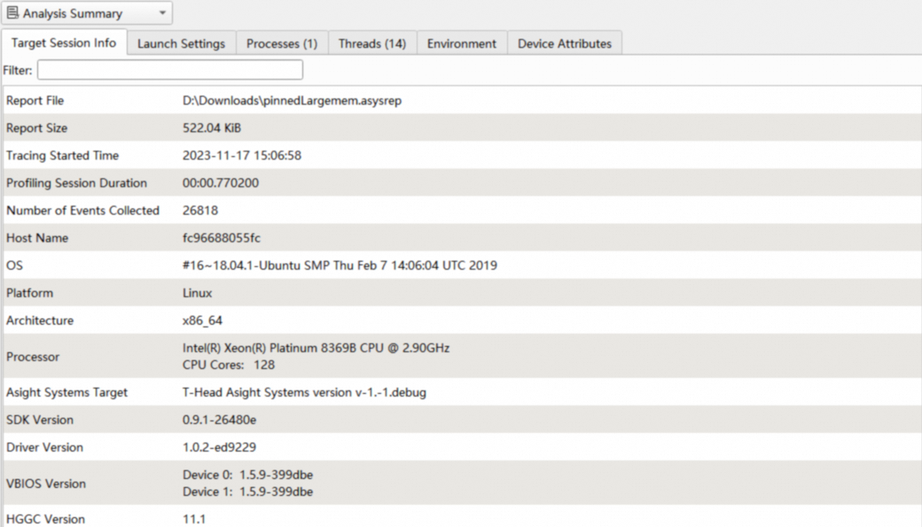
The Analysis Summary View includes the following sections:
Launch settings
Session info
Processes
Threads
Environment
Device attributes
4.1 Launch settings
The Launch Settings section shows the settings used to collect the report:
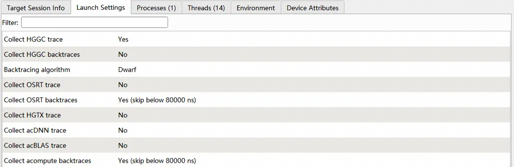
Parameter | Description |
Collect HGGC trace | Whether HGGC trace collection was enabled. |
Collect HGGC backtraces | Whether HGGC backtrace collection was enabled. |
Backtracing algorithm | The algorithm used to collect backtraces. |
Collect OSRT trace | Whether OSRT trace collection was enabled. |
Collect OSRT backtraces | Whether OSRT backtrace collection was enabled. |
Collect HGTX trace | Whether HGTX trace collection was enabled. |
Collect acDNN trace | Whether acDNN trace collection was enabled. |
Collect acBLAS trace | Whether acBLAS trace collection was enabled. |
Collect CPU samples | Whether CPU sampling was performed. |
Delay | The delay before collection started. |
4.2 Session info
The Session Info section provides details about the collection session:
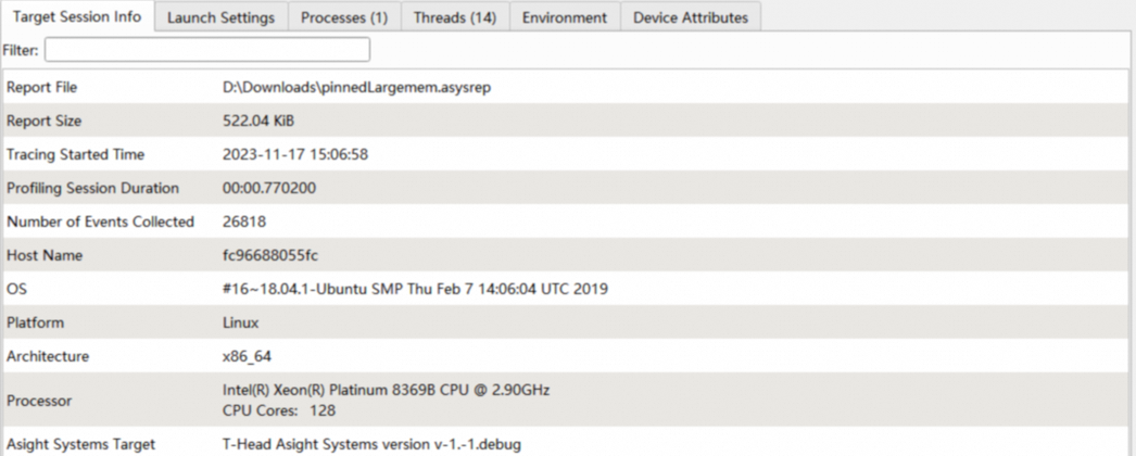
Parameter | Description |
Report file | The path to the generated report file. |
Report size | The size of the report file. |
Tracing started time | The collection start time. |
Target name | The name of the target. |
Target OS | The operating system of the target. |
Platform | The operating system platform. |
Target architecture | The architecture of the target. |
Target processor | The processor of the target. |
Asight systems target | The version of the Asight command line tool. |
CLI command used | The command-line arguments used by the Asight tool. |
4.3 Other information
The Analysis Summary View also includes the following tables:
Item | Description |
Processes | Details of the processes captured in the report. |
Threads | Details of the threads captured in the report. |
Environment | The environment variables of the PPU application. |
Device attributes | The device attributes of the PPU. |
5. Diagnostics summary
The Diagnostics Summary lists all diagnostic information in the report, including level, source, process ID, relative time, and description. The top-right corner of the Timeline View shows a cumulative overview of the diagnostic information. Click this overview to open the Diagnostics Summary View.


6. Files
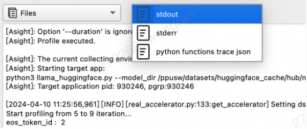
The Files view lets you inspect application log files in the report for troubleshooting. You can view logs from stdout, stderr, and python functions trace json.
Note: By default, the asys command line saves stdout and stderr to the report. The python functions trace json content appears only if you use JSON to specify its collection.
7. Connection dialog
The Asight Systems GUI provides the Connection Dialog for remote collection. Before you start, ensure that the SSH service is set up on the target machine. For instructions, see Install the SSH service. To open the Connection Dialog, go to Connection->Connect. The dialog, shown below, has three main sections:
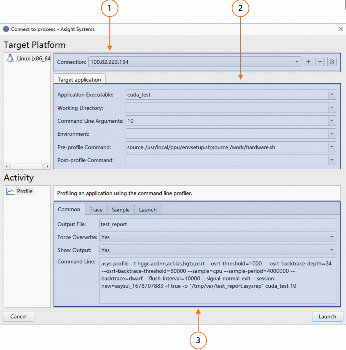
Remote connection management.
Target application configuration.
Trace collection options.
7.1 Remote connection management
Click the "+" button to add a new connection.

The remote connection configuration dialog, shown below, supports two authentication modes:
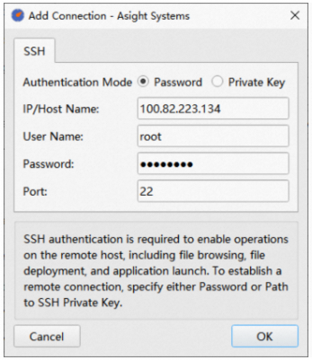
For password mode, configure the following parameters:
Parameter | Description |
IP/Host Name | IP address or hostname of the target machine. |
User Name | Username for the target machine. |
Password | Password for the target machine. |
Port | SSH port of the target machine. |
For private key mode, configure the following parameters:
Parameter | Description |
IP/Host Name | IP address or hostname of the target machine. |
User Name | Username for the target machine. |
SSH Private Key | Path to the SSH private key file. |
SSH Key Passphrase | Passphrase for the SSH private key. |
Port | SSH port of the target machine. |
7.2 Target application configuration
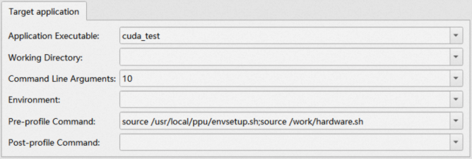
This section lets you configure launch parameters for the target application, including its path, command-line arguments, and environment variables.
Parameter | Description |
Application Executable | Path to the target application on the target machine. |
Working Directory | Working directory for the target application. |
Command Line Arguments | Command-line arguments for the target application. |
Environment | Additional environment variables for the target application. |
Pre-profile Command | A command that runs before trace collection starts. You can use this to set environment variables. |
Post-profile Command | A command that runs after trace collection ends. |
7.3 Trace collection options
Asight Systems can collect various data types, which you configure in this section.
7.3.1 Common
On the Common tab, you can set the name for the output report.
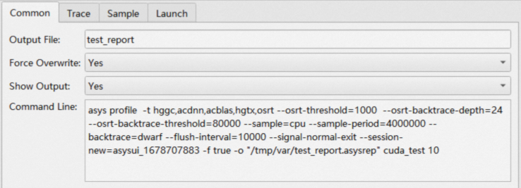
Parameter | Description |
Output File | Name of the generated report. You can specify a full path. |
Force Overwrite | If selected, overwrites an existing report with the same name. |
Show Output | If selected, displays output from the target application. |
Command Line | The |
Tip: Remote collection works by running the asys tool on the target machine to collect data and then downloading the report to your local machine. The Command Line field shows the exact command that runs on the target machine.
7.3.2 Trace
On the Trace tab, you can configure collection details for HGGC and OS runtime, and enable or disable HGTX data collection.
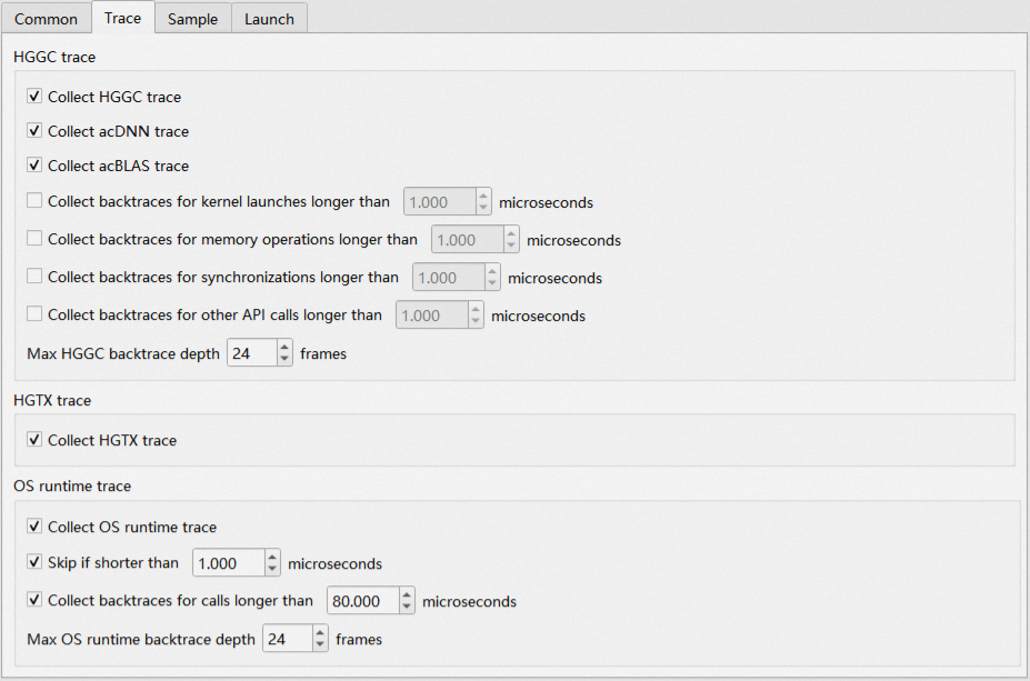
Parameter | Description |
Collect HGGC trace | Enables HGGC data collection. |
Collect acDNN trace | Enables acDNN data collection. |
Collect acBLAS trace | Enables acBLAS data collection. |
Max HGGC backtrace depth | Sets the maximum depth for HGGC backtraces. The default is 24 frames. |
Collect HGTX trace | Enables HGTX data collection. |
Collect OS runtime trace | Enables OS runtime data collection. |
Max OS runtime backtrace depth | Sets the maximum depth for OS runtime backtraces. The default is 24 frames. |
7.3.3 Sample
On the Sample tab, you can configure details for CPU sampling.
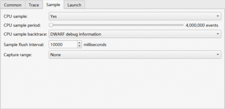
Parameter | Description |
CPU sample | Enables CPU sampling. |
CPU sample period | The CPU sampling period in CPU cycles. A smaller period results in a larger report. |
CPU sample backtrace | Enables backtrace collection for CPU samples. |
Sample flush interval | Sets the interval for flushing sample data. |
Capture range | Starts and stops trace collection based on events. |
7.3.4 Launch
On the Launch tab, you can configure manual collection triggers, the collection start time, and the duration.
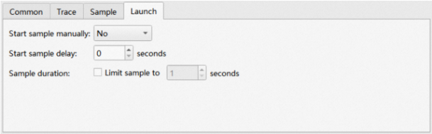
Parameter | Description |
Start sample manually | If selected, collection must be triggered manually. |
Start sample delay | Sets a delay before collection starts. |
Sample duration | Sets the duration of the collection session. |
Options
To customize the interface, open the Options dialog by selecting Tools > Options... from the menu bar.
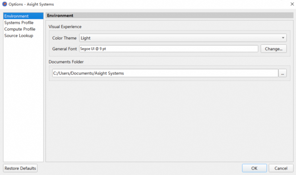
The Options dialog contains two tabs related to Asight Systems:
Environment
Systems Profile
Modified options are displayed in bold. Click the Restore Defaults button to restore the default settings.
8.1 Environment
The Environment page contains global settings for the Asight Systems GUI:
Option | Description |
Color Theme | Switches between the Light and Dark color themes. |
General Font | Changes the GUI font. |
Documents Folder | Specifies the directory for reports generated during remote collection. |
8.2 Systems profile
The options on the Systems Profile page specify the display behavior for reports:
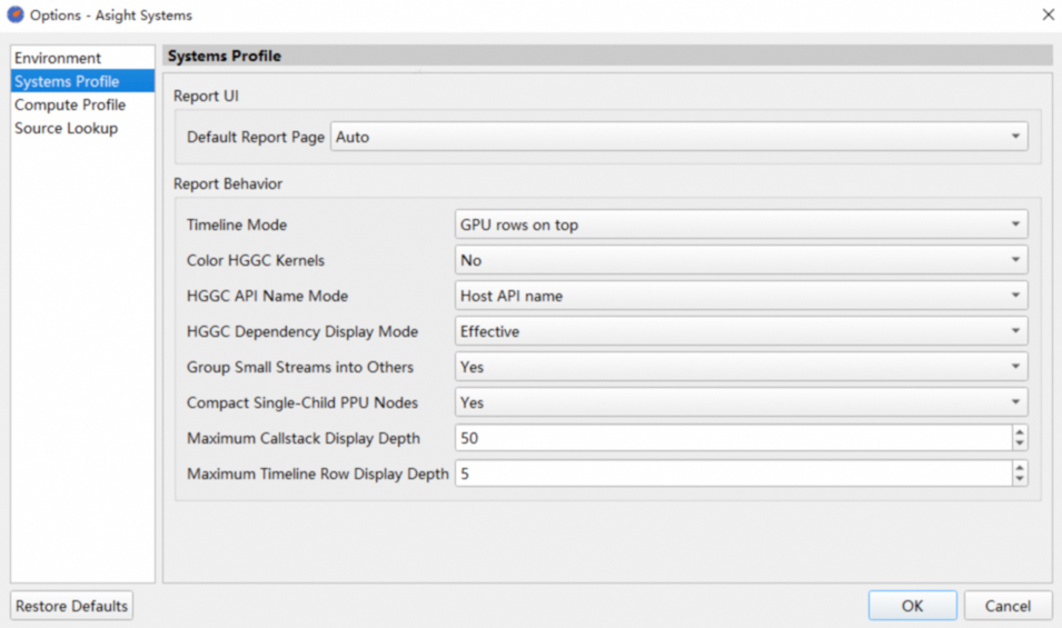
Option | Description |
Default Report Page | Specifies the page displayed when you open a report. Default: Auto, which lets Asight Systems determine the initial page. |
Color HGGC kernels | Specifies whether to display different kernels with unique colors in the Timeline View. Default: No. |
HGGC API Name Mode | When enabled, displays the HGGC launch API with its corresponding kernel name. Default: Host API name. |
HGGC Dependency Display Mode | Determines whether to calculate PPU activity dependencies from the report start time or from the corresponding host API start time. Default: Effective, which starts the calculation from the host API start time. |
Group Small Streams into Others | Specifies whether to group streams with low time percentages into an "Others" stream. Default: Yes. |
Compact Single-Child PPU Nodes | When enabled, simplifies the tree by hiding intermediate nodes with a single child. For example, if a Device node has only one Context node, the Context node is hidden and its children appear directly under the Device node. This also applies to stream nodes. Default: Yes. |
Timeline Mode | Determines the display position of PPU and CPU information. |
Maximum Call Stack Display Depth | Sets the maximum number of frames to display in a call stack. |
Maximum Timeline Row Display Depth | Sets the maximum display depth for timeline rows. Rows exceeding this depth are collapsed and can be expanded by clicking the |
 icon.
icon.