Table Document supports daily office tasks and helps financial professionals process complex financial data. This topic introduces its user interface, basic operations, and common features.
Overview
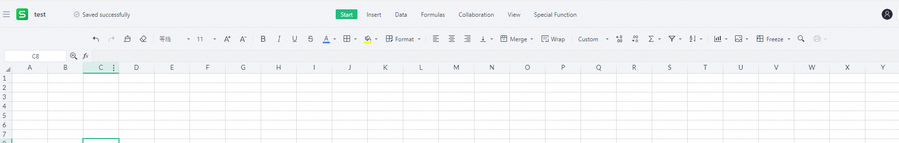
Worksheet interface
| No. | Parameter | Description |
| ① | title bar | Displays the current file name. When you create a new file, the application assigns a default name, such as workbook, workbook (1), and so on. |
| ② | ribbon | Contains the commands for editing the worksheet. |
| ③ | name box | Displays the address of the selected cell. If you select multiple cells, this box displays the selected range. |
| ④ | edit bar | Used to modify data in the active cell. It also displays content as you type directly into a cell. |
| ⑤ | column header | A worksheet consists of columns (vertical series of cells) and rows (horizontal series of cells). Columns and rows are identified by column headers and row numbers, respectively.
|
| ⑥ | row number | |
| ⑦ | active cell | A cell is the smallest unit for storing data. You can directly edit the data in the active cell. |
| ⑧ | active worksheet | A worksheet consists of cells. The tab for the active worksheet is highlighted, and you can edit its cells directly. |
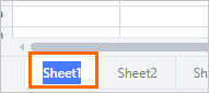
| ⑨ | worksheet tabs | Displays the names of the worksheets in a workbook. Click a tab to make a worksheet active, or double-click a tab to rename it. |
Workbooks and worksheets
Think of a workbook as a book and a worksheet as a page within that book. A workbook can contain multiple worksheets to organize different types of related data.
- WorkbookA workbook is a spreadsheet file used to calculate and store data. It can contain multiple worksheets, allowing you to organize related information within a single file. The following figure shows a workbook that contains a single worksheet.
- WorksheetYou use a worksheet to organize and analyze data. Each worksheet consists of rows and columns. By default, a new workbook contains one worksheet named Sheet1. You can add or delete worksheets as needed. The worksheet tabs at the bottom of the window identify and allow you to switch between worksheets. If not all worksheet tabs are visible, click the
 or
or  icons to scroll through the tabs, as shown in the following figure.
Cells, cell addresses, and active cells
- Cell
Each worksheet consists of a grid of rectangular boxes called cells. A cell is the most basic component of a worksheet and is the fundamental unit for entering, editing, and formatting data.
- Cell address
Each cell has a unique address, which combines its column letter and row number (e.g., A2 is the address for the cell at the intersection of column A and row 2). Cells are often referred to by their address.
- Active cellThe active cell, also called the current cell, is the cell that is currently selected in a worksheet. A heavy border, the active cell pointer, outlines the active cell. You always enter data, such as text, numbers, or formulas, into the active cell. To select a cell and make it active, click it. The address of the active cell appears in the name box, as shown in the following figure.

Basic operations
Editing cells
- Select cellsSelect cells before clearing, cutting, pasting, or moving them.
- To select a single cell, click the cell.
- To select multiple non-adjacent cells, hold down Ctrl and click each cell.
- To select a range of adjacent cells, click and drag over the cells.
- To select a range of multiple rows or columns, select a cell, then hold down Shift and click another cell to define the range.
- Copy cellsChoose one of the following methods to copy a cell:
- Move the pointer over the cell's border until it becomes a four-way arrow. Then, hold down Ctrl and drag the cell to the new location. A dashed outline indicates the copy source.
- Right-click the cell and choose Copy from the context menu. Then, right-click the destination cell and choose Paste.
- Select the cell and press Ctrl+C. Then, select the destination cell and press Ctrl+V.
- Cut cellsChoose one of the following methods to cut a cell:
- Right-click the cell and choose Cut from the context menu. Then, right-click the destination cell and choose Paste.
- Select the cell and press Ctrl+X. Then, select the destination cell and press Ctrl+V.
Editing tables
Editing a table primarily involves working with its data. Common operations include auto-filling data, creating custom lists, finding and replacing content, and entering formulas.
| Type | Description |
| text | A combination of letters, numbers, and symbols. For example, names or Grade 2005, Class A. |
| numeric | Consists of only numbers and can be used in calculations. |
- Entering text
In a table document, text refers to any combination of characters. Any entry that is not recognized as a number, formula, date, or logical value is treated as text.
Some entries, such as phone numbers or serial numbers (for example,010), look like numbers but should be treated as text because they are not used in calculations. If you enter010as a number, the leading zero is dropped. To preserve entries like these, treat them as text.- To enter a number as text, type a single quotation mark (') before the number.
- You can drag the fill handle to fill a series. To copy the data instead, hold down Ctrl while dragging the fill handle.
- Entering numbersNumbers can include the digits 0-9 and special characters such as
+`, `-`, `$`, and `%.Note Note the following when entering numbers:- You do not need to type a plus sign (+) for positive numbers.
- A number enclosed in parentheses is treated as a negative number. For example,
(123)is interpreted as -123. - To prevent a fraction like 1/2 from being converted to a date, type
0 1/2(with a space between the 0 and the fraction). If you enter just1/2, it is interpreted as a date (for example, January 2). - If a number is too long to fit in the cell's width or exceeds 11 digits, it is automatically displayed in scientific notation.
- Entering dates and times
- To enter a date, use slashes (/) or hyphens (-) to separate the year, month, and day, such as
05/4/19or05-4-19. - To enter a time, use colons (:) to separate hours, minutes, and seconds, such as
9:30or10:30 AM.
Note Dates and times are treated as numbers, so you can perform calculations with them. - To enter a date, use slashes (/) or hyphens (-) to separate the year, month, and day, such as
- Entering the same data in non-adjacent cellsTo do this:
- Hold down Ctrl and select the desired non-adjacent cells.
- Type the data in the active cell and press Ctrl+Enter to apply it to all selected cells.
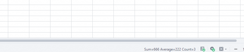
- Viewing summary calculations on the status barThe status bar provides useful information about selected data. If you select a range of cells containing numbers, the status bar automatically displays their Sum, Average, and Count, as shown in the following figure.
Note The calculations shown are the default settings. You can right-click the status bar to add or remove items from the display.
Cut, copy, and paste
You can cut, copy, and paste selected content using menu commands, keyboard shortcuts, or your mouse.
Cut
The cut command removes the selected content from its location and places it on the system clipboard. You can then paste the content in a different location.
- Press Ctrl+X.
- Right-click the selection and select Cut from the context menu.
Copy
The copy command places a duplicate of the selected content on the system clipboard, leaving the original content in place. You can then paste the content in a different location.
- Press Ctrl+C.
- Right-click the selection and select Copy from the context menu.
Paste
The paste command inserts content from the system clipboard at the cursor. This command is only available when the system clipboard contains content.
- Press Ctrl+V to paste the cut or copied content.
- Right-click at the destination and select Paste from the context menu.
Format painter
The format painter copies formatting from a selected object, text, or cell and applies it to another.
- Select the content (such as an object, text, or cell) with the formatting you want to copy.
- On the Start ribbon, click the icon.
- When the pointer changes to a paintbrush shape, select the object, text, or cell you want to format.
 icon to apply the same format to multiple selections.
Font settings
Apply different font formats, borders, and fill colors to cells to make important content stand out.
Font formats
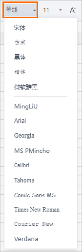
- Set the font
- Select the cell or text you want to format.
- On the Start ribbon, click the font drop-down list and select a font.
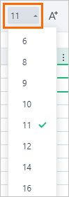
- Set the font sizeThe font size determines how large the characters appear.
- Select the cell or text you want to format.
- On the Start ribbon, click the font size drop-down list and select a font size.
Note On the Start ribbon, you can also click the icon to increase the font size or the icon to decrease it. - Set the font styleThe Start ribbon provides several icons to apply common font styles. These icons and their functions are described in the following table.
Icon Function Applies or removes bold formatting. Applies or removes italics. Applies or removes an underline. Applies or removes a strikethrough. Click the arrow next to the icon and select a text color.
 icon to increase the font size or the
  icon to decrease it.


 next to the icon and select a text color.
Cell borders
By default, worksheet gridlines are gray and do not print. To print the gridlines, add borders to the worksheet.
- Select the cell or cells where you want to add a border.
- On the Start ribbon, click the drop-down arrow next to the icon and select the border you want.
- Click the drop-down arrow next to the icon and select a color for the border.
- Click the drop-down arrow next to the icon and select a style for the border.
 icon and select the border you want.
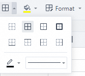
 icon and select a color for the border.
 icon and select a style for the border.
Cell fill
- On the Start ribbon, click the drop-down arrow next to the icon and select a color.
- Select the cell you want to fill, right-click, and select Format Cells from the right-click menu. In the panel on the right, select the Cell tab and set a fill color.
 icon and select a color.
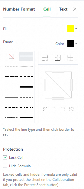
Align, wrap, and merge cells
Align cells
Alignment determines how content is positioned within a cell. By default, text is left-aligned, numbers are right-aligned, and logical values and error values are centered. You can also apply other alignment settings to the content in your cells.
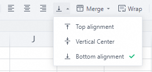
- Select the cell or cells you want to align.
- On the Home ribbon, click an alignment option.
Icon Description align left center align right top align middle align bottom align


Wrap text
- Select the cell or cells where you want to wrap text.
- On the Home ribbon, click the icon.
 icon.
icon.Merge cells
- Select the cells you want to merge.
- On the Home ribbon, click the drop-down arrow to the right of the icon and select a merge option.
Icon Description Merges the selected cells and centers the content. Merges selected cells with identical content. Merges the content of the selected cells. Merges cells in each row of the selection. Unmerges the selected cell. Note You can also click the merge icon again to unmerge cells.
 icon and select a merge option.
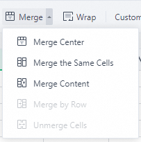


Format cells
Quick formatting
On the Start ribbon, click the  icon to increase the number of decimal places for higher precision, or click the
  icon to decrease it for lower precision.
Cell formats
You can format cells using 13 categories: general, number, currency, accounting, short date, long date, time, percentage, fraction, scientific notation, text, comma style, and custom.
- Select the cells you want to format.
- On the Start ribbon, click the drop-down arrow to the right of the icon, and select a format from the drop-down list. The following table describes the available formats.
Icon Description The default cell format. It has no specific number format. Displays the number with two decimal places. Displays numbers with a currency symbol. For example: $4.00. Aligns currency symbols and decimal points in a column. Displays the date in a short format, such as 8/31/2018. Displays the date in a long format, such as August 31, 2018. Displays time values, for example, 12:00:00 AM. Multiplies the cell value by 100 and displays the result with a percent sign (%). Displays the number as a fraction, for example, 1/8. Displays the number in scientific notation, for example, 1.23E+09. Treats the content of a cell as text, even when a number is in the cell. Adds a thousands separator to the number. Lets you create a custom number format based on an existing one.
 icon, and select a format from the drop-down list. The following table describes the available formats.


Style settings
Table style
Table Document offers a variety of built-in table styles. Select a style that fits your data to quickly format your table. Each table style applies a unique set of formatting, such as font weight, border thickness, and background color, to different rows and columns.
 icon and select a table style, as shown in the following figure.
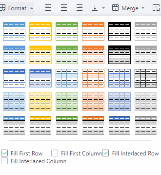
Conditional formatting
Conditional Format automatically applies specific formats to cells when certain conditions are met. You can define up to three conditions at once, based on either a formula or a cell value. For example, you can highlight a cell in yellow if its value matches the current date.
- Select the cells you want to format.
- On the Data ribbon, click the icon to open the Conditional Format panel, as shown in the following figure.
- Click the drop-down arrows next to the and icons and select a condition from the lists.
- In the Format Style section, click the drop-down arrow to select the format to apply.
- Click Create Rule.
 icon to open the Conditional Format panel, as shown in the following figure.
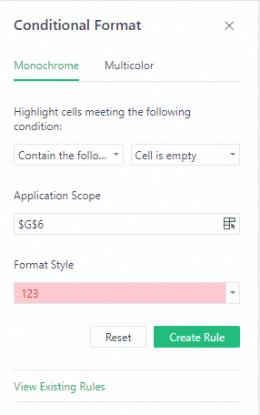
 and
and  icons and select a condition from the lists.
Cell Settings
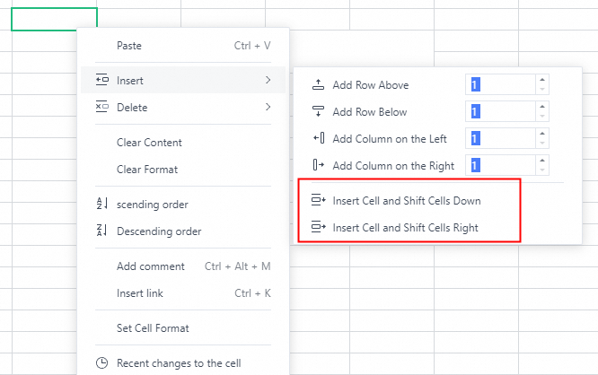
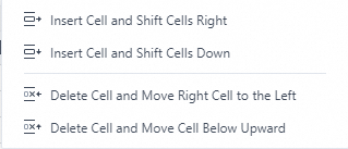
Inserting cells
- Method 1:
- Select the cell or range where you want to insert new cells.
- On the Insert ribbon, click the icon and select an insertion option.
- Method 2:
- Select the cell or range where you want to insert new cells.
- Right-click the selection.
- In the right-click menu, click Insert and select an insertion option.
 icon and select an insertion option.
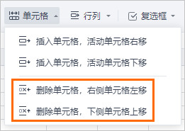
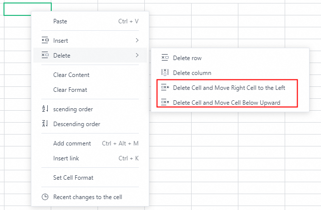
Deleting cells
- Method 1:
- Select the cell or cells to delete.
- On the Home ribbon, click the icon and select a deletion option.
- Method 2:
- Select the cell or cells to delete.
- Right-click the selection.
- In the right-click menu, click Delete and select a deletion option.
Row and column settings
You can change the structure of a spreadsheet by selecting, inserting, and deleting rows and columns.
Select rows and columns
- To select a single row or column, click the row number or column header.
- To select a range of adjacent rows or columns, click the first row number or column header, hold down the Shift key, and then click the last row number or column header in the range.
- To select non-adjacent rows or columns, hold down the Ctrl key and click each desired row number or column header.
Hide and unhide rows and columns
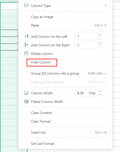
- To hide rows or columns:
- Select the rows or columns you want to hide.
- Right-click the selection.
- Click Hide Row or Hide Column.
- To unhide rows or columns:
- Click the Select All icon in the upper-left corner to select the entire worksheet.
- Right-click anywhere in the selection.
- Click Unhide Row or Unhide Column.
- Click the Select All icon
 in the upper-left corner to select the entire worksheet.
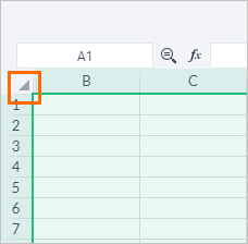

Insert rows and columns
- Method 1:
- Select where you want to insert a new row or column.
- On the Insert tab, click the icon, then click Insert Row or Insert Column.
- Method 2:
- Select where you want to insert a new row or column.
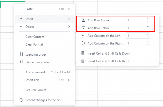
- Right-click the selection.
- Click Insert Row or Insert Column.
 icon, then click Insert Row or Insert Column.
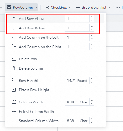
Delete rows and columns
- Method 1:
- Select the rows or columns you want to delete.
- On the Insert tab, click the icon, then click Delete Row or Delete Column.
- Method 2:
- Select a cell in the row or column you want to delete.
- Right-click the cell.
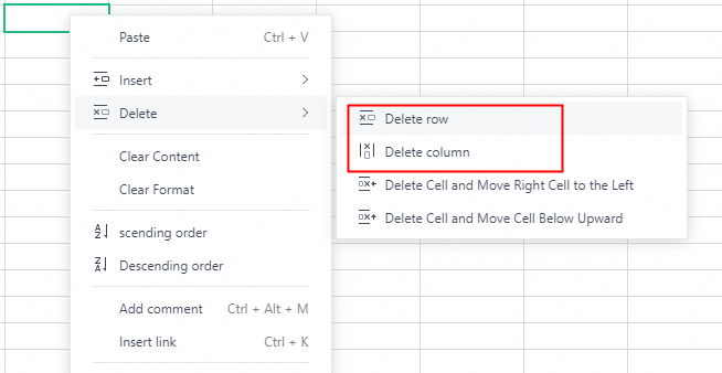
- Click Delete, then click Delete Row or Delete Column.
- Method 3:
- Select the rows or columns you want to delete.
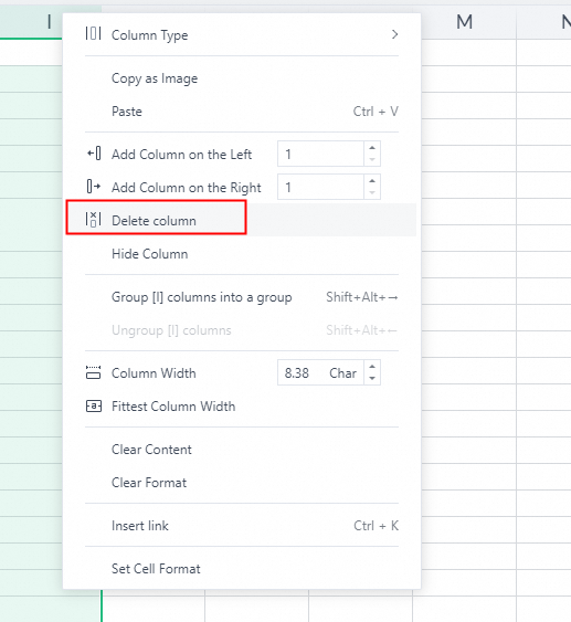
- Right-click the selection.
- Click Delete.
 icon, then click Delete Row or Delete Column.
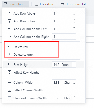
Set row height or column width
- Method 1:
- Select the rows or columns that you want to resize.
- On the Insert tab, click the icon, then click Row Height or Column Width.
- Method 2:
- Select the rows or columns that you want to resize.
- Right-click the selection.
- Click Row Height or Column Width.
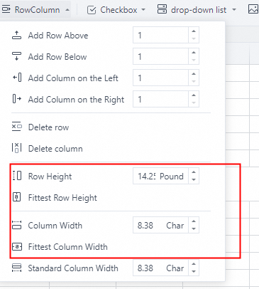
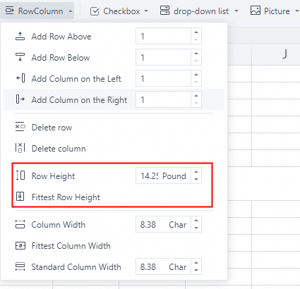
- Selecting Fittest Row Height or Fittest Column Width automatically adjusts the row height or column width to fit the content.
- Selecting Standard Column Width sets a uniform column width for the current worksheet, excluding any columns that have been manually resized.
Worksheet settings
A workbook can contain multiple worksheets. You can insert, duplicate, move, delete, rename, and hide worksheets within a workbook.
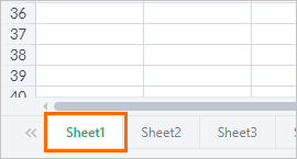
Select worksheet
Move worksheet
- Drag and drop the worksheet tab.
- Press and hold the left mouse button on the worksheet tab you want to move.
- Drag the tab to the desired location, and then release the mouse button.
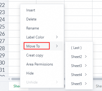
- Use the Move To feature.
- Right-click the worksheet tab you want to move.
- From the right-click menu, click Move To and select a new position for the worksheet.
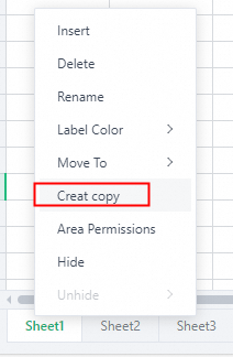
Duplicate worksheet
- Right-click the worksheet tab you want to duplicate.
- From the right-click menu, click Duplicate.
Create or insert worksheet
- Create a new worksheet
Click the
icon to the right of the worksheet tabs. - Insert a worksheetTo insert a worksheet:
- Right-click the active worksheet's tab.
- From the right-click menu, click Insert.
 icon to the right of the worksheet tabs.
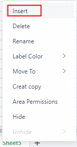
Delete worksheet
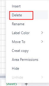
- Right-click the worksheet tab you want to delete.
- From the right-click menu, click Delete.
- In the delete worksheet dialog box, click OK.
Rename worksheet
Sheet + number. To rename a worksheet, do one of the following:- Method 1:
- Double-click the worksheet tab you want to rename. When the tab is highlighted, enter a new name.
- Press Enter or click anywhere in the worksheet except the worksheet tab.
- Double-click the worksheet tab you want to rename. When the tab is highlighted, enter a new name.
- Method 2:
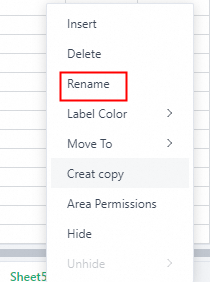
- Right-click the worksheet tab you want to rename.
- From the right-click menu, click Rename and enter a new name.
- Press Enter or click anywhere in the worksheet except the worksheet tab.
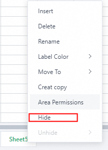
Hide worksheet
- Right-click the worksheet tab you want to hide.
- From the right-click menu, click Hide.
Edit a table
Fill
- Autofill dataUse the autofill feature to enter data quickly and efficiently using copy fill or fill series.
- Copy fillTo perform a copy fill:
- Enter content in a cell, then select the cell.
- Move the pointer over the fill handle in the lower-right corner of the cell until it changes to a plus sign (+).
- Hold down Ctrl, then click and drag the fill handle downward.
- Release the mouse button after dragging the fill handle to the last cell you want to fill.
- Fill seriesThe application supports two common types of series:
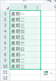
- Text series: such as years, months, weekdays, and quarters.The following example shows how to fill a series of weekdays:
- Enter Monday in the first cell, then select the cell.
- Move the pointer over the fill handle in the lower-right corner of the cell until it changes to a plus sign (+).
- Click and drag the fill handle downward.
- Release the mouse button after dragging the fill handle to the last cell you want to fill, as shown in the following figure.
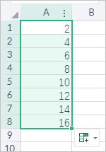
- Numeric series: such as 1, 2, 3 or 2, 4, 6.For a numeric series, enter at least two numbers to establish a pattern, then drag the fill handle to continue the series.
- Enter 2 in the first cell and 4 in the second cell, then select both cells.
- Move the pointer over the fill handle in the lower-right corner of the selection until it changes to a plus sign (+).
- Click and drag the fill handle downward.
- Release the mouse button after dragging the fill handle to the last cell you want to fill, as shown in the following figure.
- Text series: such as years, months, weekdays, and quarters.
- Copy fill
- Smart fill data (Ctrl+E)Use the Ctrl+E keyboard shortcut to perform a smart fill. Smart fill is useful for the following tasks:
- Extract an item from a string.
- Combine multiple columns into one column.
- Convert case and reorder strings.
- Clean and standardize data.
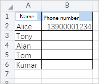
The following example shows how to use smart fill to extract phone numbers:- In the column next to your data, enter an example of the phone number you want to extract, as shown in the following figure.
- Select the cell below your sample, then press Ctrl+E. Alternatively, on the Data ribbon, click the icon. Smart fill automatically extracts and fills the phone numbers into the column, as shown in the following figure.
 icon. Smart fill automatically extracts and fills the phone numbers into the column, as shown in the following figure.
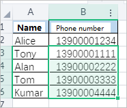
Clear formatting or content
- Clear formattingTo clear the formatting from cells:
- Select the cells with the formatting you want to remove, then right-click the selection.
- From the right-click menu, choose Clear Format. This removes the cell's formatting but keeps its content.
- Clear contentTo clear the content from cells:
- Select the cells with the content you want to remove, then right-click the selection.
- From the right-click menu, choose Clear Content. This removes the cell's content but keeps its formatting.
Sort and filter
- SortSorting lets you organize your data by arranging rows or columns in ascending or descending order. To sort data:
- Select a cell in the data range you want to sort.
- On the Home ribbon, click the icon and choose a sort option, as shown in the following figure.
- FilterFiltering is a quick way to find and work with a subset of data in a list. It displays only the rows that meet the criteria you specify. Unlike sorting, filtering does not reorder the list; it temporarily hides the rows you do not want to see. To filter data:
- Select a cell in the data range you want to filter.
- On the Home ribbon, click the icon.
- A filter arrow appears in the header of each column. Click the arrow to display a list of filter options. The following example shows how to filter by year.
 icon and choose a sort option, as shown in the following figure.
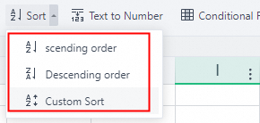
 icon.
icon.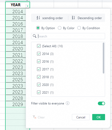
Find and replace
- Find cell contentTo find content in a cell:
- On the Home ribbon, click the icon to open the Find & Replace dialog box, as shown in the following figure.
- In the Find what text box, enter the content you want to find.
- Press Enter or click Find to start the search.Note
- If the content is not found in the selected range, the message No data matching the query content was found appears.
- Click the or icons next to the text box to navigate to the previous or next match.
- On the Home ribbon, click the
- Replace cell contentThe replace feature lets you quickly modify your worksheet by replacing content that meets your criteria. To replace cell content:
- On the Home ribbon, click the icon to open the Find & Replace dialog box.
- Click the icon to show the replace options, as shown in the following figure.
- In the Find what text box, enter the content you want to find. In the Replace with text box, enter the replacement content.Important If you leave the Replace with text box empty, the operation deletes the found content.
- Click Replace All to replace all matches.
- On the Home ribbon, click the
 icon to open the Find & Replace dialog box, as shown in the following figure.
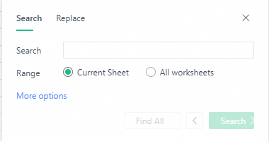
 or
or  icons next to the text box to navigate to the previous or next match.
 icon to show the replace options, as shown in the following figure.
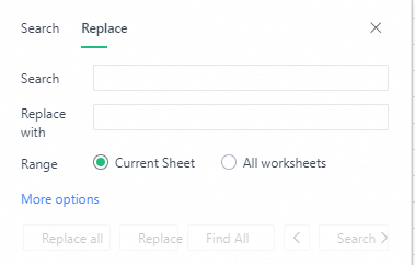
Insert an image
Insert an image into a table to better visualize data and clarify its meaning.
- Insert an image in one of the following ways:
- On the Start ribbon, click the icon and select Image from the drop-down list.
- On the Insert ribbon, click the icon.
- On the Start ribbon, click the
- Select the image type.
- floating picture: The image floats over cells.
- cell picture: The image is placed inside a cell.
Note Click When pasting pictures from outside to set a default: Default to floating picture or Default to cell picture. - In the Open dialog box, locate and select the image file you want to insert.
- Click Open to insert the image.
 icon and select Image from the drop-down list.
 icon.
icon.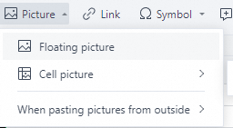
Insert link
You can add a link to a cell to quickly access a web page.
- Select the cell where you want to insert the link.
- On the Insert ribbon, click the icon.
- In the Insert Link dialog box, set the following options:
- Text: Enter a name for the link.
- Type: From the drop-down list, select Link, then enter the web address in the text box.
- Click OK.
 icon.
icon.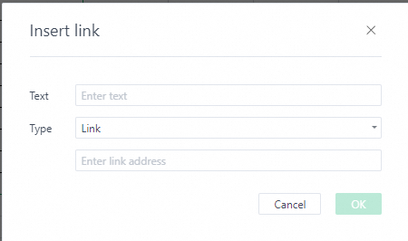
- To convert a web address in a cell into a hyperlink, right-click the cell and select Insert Link from the context menu.
- To select a linked cell, hold down Ctrl and click the cell.
- To edit a link's display text, hold down Ctrl and double-click the cell.
Insert a symbol
The insert symbol feature in Table Document lets you add symbols that aren't on your keyboard, such as Greek letters, mathematical symbols, and graphic symbols.
- Select the cell where you want to insert the symbol.
- On the Insert ribbon, click the icon and select a symbol.
 icon and select a symbol.
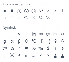
Insert a checkbox
Use checkboxes to mark items as complete or track task status.
- Select the cell range where you want to insert checkboxes.
- On the Insert ribbon, click the icon to insert the checkboxes. By default, the checkboxes are unchecked.
- (Optional) To remove checkboxes, select the cells containing them. Then, on the Insert ribbon, click the drop-down arrow next to the icon and select Clear the checkbox.
 icon to insert the checkboxes. By default, the checkboxes are unchecked.
Insert PivotTable
A PivotTable is a powerful tool for calculating, summarizing, and analyzing data. It helps you see comparisons, patterns, and trends in your data.
- Select a cell range that contains data in the worksheet.
- On the Insert ribbon, click the icon.
- In the Create PivotTable dialog box, select a location for the PivotTable.
- Click OK.
- Select the PivotTable range. In the pane on the right, click the icon, then add the data columns to the corresponding row, column, and value areas.
 icon.
icon.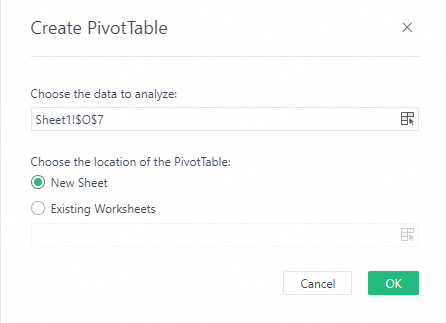
 icon, then add the data columns to the corresponding row, column, and value areas.
 icon in the upper-right corner of a field to select a different calculation method, such as count, maximum value, or variance.
Page zoom
You can adjust a spreadsheet's zoom level. Zoom in for a closer view of the worksheet, or zoom out to see more of it. The supported zoom range is 50% to 400%.
 icon in the lower-right corner of the page and select a percentage from the Display Ratio list.
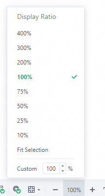
Formula settings
A formula is an equation for analyzing and calculating data in a worksheet. Table Document provides a rich library of functions to create formulas for calculations like addition, subtraction, multiplication, and division.
Table Document supports more than 300 functions across nine categories, including Date and time, Math and trigonometry, Statistical, Lookup and reference, Text, Logical, and Information.
AutoSum
The AutoSum feature in Table Document simplifies summing data in a worksheet.
- Sum a rowTo sum a row, follow these steps:
- Select the row of cells you want to sum.
- On the Start ribbon, click the drop-down arrow to the right of the icon.
- From the drop-down list, select Sum.
- The AutoSum result appears in the cell immediately to the right of the selected range, as shown in the following figure.
- Sum a columnTo sum a column, follow these steps:
- Select the column of cells you want to sum.
- On the Start ribbon, click the drop-down arrow to the right of the icon.
- From the drop-down list, select Sum.
- The AutoSum result appears in the cell immediately below the selected range, as shown in the following figure.
 icon.
icon.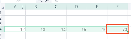
Error checking
- An error indicator appears when a formula in a worksheet cell returns an error. This indicator is a small green triangle in the top-left corner of the cell, with an icon to its left, as shown in the following figure.
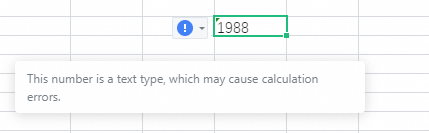
- Hover over the icon to view the error type, as shown in the following figure.
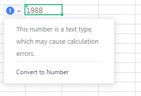
- Click the icon to view the error type and correction options, as shown in the following figure.
- Hover over the
- Supported error types:
- Error Values: An error indicator appears if the formula returns an error value, such as #VALUE! or #DIV/0!.
- Number stored as text (correction available): This error occurs when a cell contains a number stored as text. An error indicator with correction options appears. For example, in Table Document, the number 1 and the text "1" are treated differently.
- Inconsistent formula in a range (correction available): This error occurs when a formula in a cell does not match the pattern of formulas in adjacent cells.
- Formula omits cells in a range (correction available): This error occurs when a formula referencing a data range omits contiguous cells within it. For example, if cells A1:A100 contain data and the formula is =SUM(A1:A98), this error will be triggered.
- Formula refers to empty cells: An error indicator appears if the formula references an empty cell.
- Data validation: After you set data validation rules, an error indicator appears in cells with existing data that violates the validation criteria.
 icon to its left, as shown in the following figure.
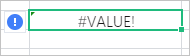
Calculation
A calculation evaluates a formula and displays the resulting value in a cell. By default, Table Document automatically recalculates workbooks that contain formulas when you open them. Table Document offers several calculation methods to control how data is processed, including automatic recalculation, iterative calculation, and manual recalculation.
Configure workbook recalculation
Table Document uses automatic recalculation by default. If a workbook contains complex circular references, you can switch to manual recalculation. Follow these steps:- On the Formulas ribbon, click the icon.
- In the Options dialog box, select manual recalculation, as shown in the following figure.
- Click OK.
 icon.
icon.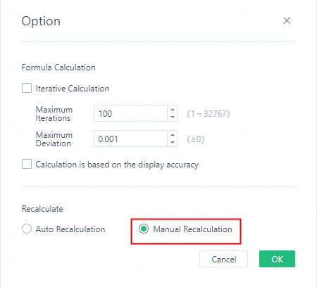
manual recalculation is enabled, Table Document does not automatically recalculate formulas when you change data in a worksheet. To update the calculations, click the  icon on the Formulas ribbon to recalculate all
 formulas in the workbook.Configure iterative calculation
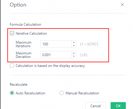
Iterative calculation repeatedly recalculates formulas until a specific number of iterations is met or the results converge within a specified limit. This feature resolves circular references, which occur when a formula refers back to its own cell, either directly or indirectly.
iterative calculation, follow these steps:- On the Formulas ribbon, click the icon.
- In the Options dialog box, select the iterative calculation checkbox, then enter values for maximum iterations and maximum deviation, as shown in the following figure.
- Click OK.
Set precision as displayed
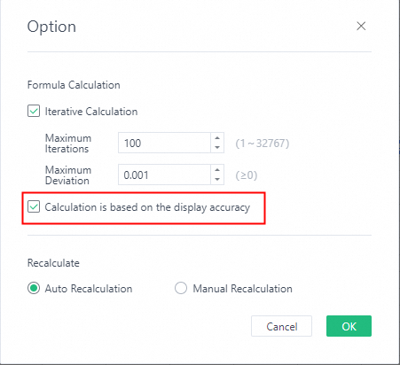
By default, Table Document uses the full underlying value of a cell for calculations, not the formatted or displayed value. This can cause discrepancies between a calculated result and a manual sum of the displayed values. To resolve this, enable the precision as displayed option. This forces all calculations in the workbook to use the displayed, rounded value of each cell.
precision as displayed, follow these steps:- On the Formulas ribbon, click the icon.
- In the Options dialog box, select the precision as displayed checkbox, as shown in the following figure.
- Click OK.
Names
A name is a user-defined alias for a cell, range, or formula. You can use this name in other formulas to refer to the underlying value or result.
Naming rules
- Names can contain uppercase and lowercase letters, but they are not case-sensitive. For example, if you have already created the name
ABC, creating another nameabcin the same document is not allowed. - Names cannot contain numbers, spaces, or punctuation marks other than underscores and periods.
- Names cannot be the same as a cell address.
- You can use underscores (_) and periods (.) as word separators.
Create a name
- Select the range to name.
- On the Formulas ribbon, click the icon. The Name Management panel opens on the right.
- In the Name Management panel, click Create Name and enter a name.
- Click OK.
- (Optional) Select the new name and click the icon in the upper-right corner to edit or delete it.
 icon. The Name Management panel opens on the right.
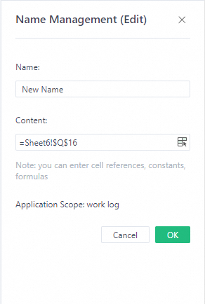
 icon in the upper-right corner to edit or delete it.
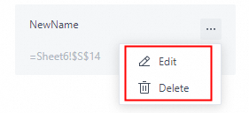
Use a name
SummaryArea=$A$1:$A$12, you can write the formula as =SUM(SummaryArea)*0.2. This is equivalent to =SUM($A$1:$A$12)*0.2.Data tools
Data validation
To ensure the accuracy and consistency of data entry, use data validation to check data in real time. This feature prevents invalid input by restricting the data types or values users can enter into a cell, improving overall efficiency.
- Select the cell or range of cells where you want to apply data validation.
- On the Data ribbon, click the icon to open the Data Validation dialog box.
- On the Settings tab, set the validation criteria.
- On the Error Alert tab, customize the error message for invalid entries.
- Click OK.
 icon to open the Data Validation dialog box.
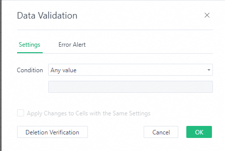
Duplicates
This feature helps you find and manage redundant data by highlighting or deleting duplicate values in a row or column.
 icon, then select Highlight Duplicates or Delete Duplicates from the drop-down list.
- Highlight Duplicates: Highlights cells with duplicate values in a selected row or column by applying a background color.
- Delete Duplicates: Removes duplicate values from a selected row or column, keeping only the first occurrence of each value.
Comments
In a spreadsheet, you can use comments to annotate a cell. When you add a comment to a cell, a small red triangle appears in its upper-right corner. Hover over the cell to view the comment.
Add comment
You can add comments to a cell or a range of cells to leave notes or reminders.
- Select the cell where you want to add a comment.
- Open the comment text box in one of the following ways:
- On the Insert ribbon, click the icon.
- Right-click the cell and select Add comment from the context menu.
- On the Insert ribbon, click the
- Enter your comment in the text box. Press Alt+Enter to insert a line break.
- To post the comment, click Comment or press Enter.
 icon.
icon.Edit comment
You can edit the content of an existing comment.
- Hover over the commented cell to display the comment.
- Click the icon in the upper-right corner of the comment box and select Edit, as shown in the following figure.
- Update the comment and click Save.
 icon in the upper-right corner of the comment box and select Edit, as shown in the following figure.
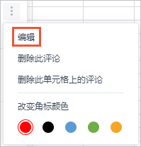
Delete comment
You can delete comments that are no longer needed.
- Hover over the commented cell to display the comment.
- Click the icon in the upper-right corner of the comment box and select Delete this comment, as shown in the following figure.
Note Click Delete All to remove all comments from this cell.

Freeze Panes
When working with a large worksheet, freeze panes to lock specific rows and columns. This keeps headers visible as you scroll.
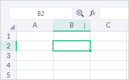
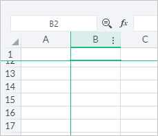
- In the worksheet, select the cell below the rows and to the right of the columns you want to freeze. For example, to freeze the first row and first column, select cell B2, as shown in the following figure.
- On the Insert ribbon, click the icon, or on the View ribbon, click the icon.
- From the drop-down list, select Freeze Panes, as shown in the following figure.
Note You can also select freeze first row or freeze first column to lock only the top row or the first column.
- The frozen rows and columns now remain fixed as you scroll through the worksheet.
- (Optional) To unfreeze panes, click the icon on the Insert ribbon or the icon on the View ribbon, and select Unfreeze from the drop-down list.
 icon, or on the View ribbon, click the
 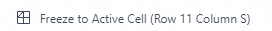 icon.
icon.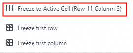
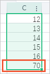
Group
Grouping rows or columns helps you manage and view specific data subsets in a large worksheet.
- Method 1:
- Select the rows or columns that you want to group.
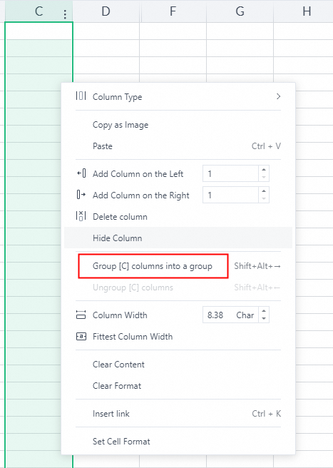
- Right-click and select Group from the shortcut menu. The figure below shows an example of grouping column C.
- Method 2:
- Select the rows or columns that you want to group.
- On the Insert ribbon, click the icon and select Group. The figure below shows an example of grouping column C.
 icon and select Group. The figure below shows an example of grouping column C.
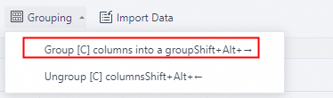
 icon or the
  icon to collapse or expand the group.
Table Document lets you print online files directly from your browser.
- On the Start ribbon, click the icon. The Print dialog box appears.
- Select Current Worksheet or All Worksheets as the print range. Click Page Settings to configure more print parameters.
- Click Next to open your browser's print window.Note If your browser cannot print, you can download the file as a PDF and print it.
 icon. The Print dialog box appears.
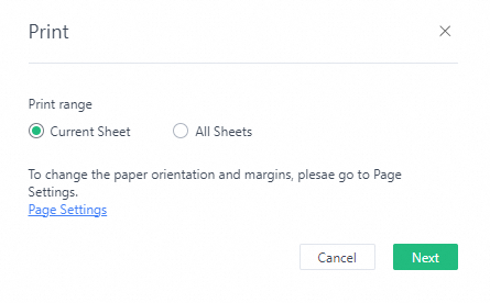
Export files
Export as image
You can export a document as an image.
- On the Efficiency ribbon, click the icon to open the Export as Image panel.
- Select the export method and export format.
- Click Export to download the image.
 icon to open the Export as Image panel.
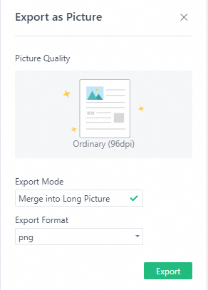
Export as PDF
You can also export a document as a PDF.
- On the Efficiency ribbon, click the icon to open the Export as PDF panel.
- Select the export range and export options.
- Click Export to download the PDF.
 icon to open the Export as PDF panel.
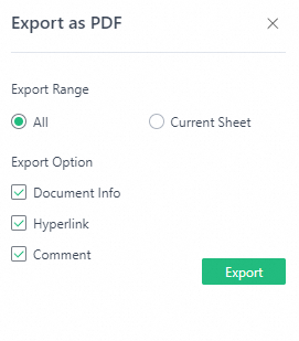
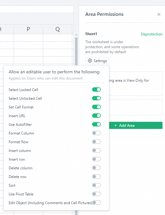
Area permissions
When collaborating, the area permission feature protects a cell range from unintended modifications. It provides precise control to prevent information leaks, reduce interference, and protect private data in collaborative tables.
- On the Collaboration ribbon, click the icon to open the Area Permissions panel.
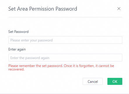
- In the Area Permissions panel, click Enable to open the Set Area Permission Password dialog box.
- Set a password, and then click OK.
- In the Area Permissions panel, click Add Area to define an editable cell range.
- After defining the editable cell ranges, click the icon to further restrict what collaborators can edit.
 icon to open the Area Permissions panel.
 icon to further restrict what collaborators can edit.