The Vertex Clustering Coefficient measures how tightly a node's neighbors are connected to each other — that is, the likelihood that any two of a node's neighbors are also directly connected. It is the ratio of actual edges among a node's neighbors to the maximum possible edges between them.
The coefficient ranges from 0 to 1:
-
0: None of the node's neighbors are connected to each other (e.g., the hub of a star network).
-
1: All of a node's neighbors are fully connected to each other (e.g., any node in a fully connected network).
How it works
For each node u in an undirected graph, the clustering coefficient is:
$$C_u = \frac{2T(u)}{deg(u)(deg(u)-1)}$$
Where:
-
T(u) — the number of triangles passing through node u (pairs of neighbors that are also directly connected to each other)
-
deg(u) — the degree of node u (number of direct neighbors)
Network topology examples
The algorithm produces boundary values on two canonical graph structures:
| Network type | Clustering coefficient | Why |
|---|---|---|
| Star network | 0 (for the central node) | Peripheral nodes connect only to the center, not to each other. |
| Fully connected network | 1 (for all nodes) | Every possible connection between neighbors exists. |
Configure the component
Method 1: Configure the component on the pipeline page
Add a Vertex Clustering Coefficient component on the pipeline page and configure the following parameters:
| Category | Parameter | Description |
|---|---|---|
| Fields Setting | Start Vertex | The start vertex column in the edge table. |
| End Vertex | The end vertex column in the edge table. | |
| Parameters Setting | Largest Vertex Degree | Nodes with a vertex degree larger than this value are sampled instead of fully computed. Default: 500. |
| Tuning | Workers | Number of workers for parallel execution. Higher values increase parallelism but also increase framework communication overhead. |
| Memory Size per Worker (MB) | Maximum memory per worker. Default: 4096 MB. If memory usage exceeds this value, an OutOfMemory error is reported. |
|
| Data Split Size (MB) | Size of each data split. Default: 64 MB. |
Method 2: Configure the component by using PAI commands
Run the Vertex Clustering Coefficient algorithm using the NodeDensity PAI command via the SQL Script component. For details on running PAI commands in SQL Script, see Scenario 4: Execute PAI commands within the SQL script component.
PAI -name NodeDensity
    -project algo_public
    -DinputEdgeTableName=NodeDensity_func_test_edge
    -DfromVertexCol=flow_out_id
    -DtoVertexCol=flow_in_id
    -DoutputTableName=NodeDensity_func_test_result
-DmaxEdgeCnt=500;| Parameter | Required | Default | Description |
|---|---|---|---|
inputEdgeTableName |
Yes | — | Name of the input edge table. |
inputEdgeTablePartitions |
No | Full table | Partitions to read from the input edge table. |
fromVertexCol |
Yes | — | Start vertex column in the input edge table. |
toVertexCol |
Yes | — | End vertex column in the input edge table. |
outputTableName |
Yes | — | Name of the output table. |
outputTablePartitions |
No | — | Partitions in the output table. |
lifecycle |
No | — | Lifecycle of the output table. |
maxEdgeCnt |
No | 500 | Nodes with a vertex degree greater than this value are sampled. |
workerNum |
No | — | Number of workers for parallel execution. |
workerMem |
No | 4096 | Maximum memory per worker (MB). An OutOfMemory error is reported if exceeded. |
splitSize |
No | 64 | Data split size (MB). |
Example
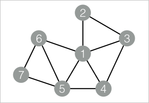
This example runs the Vertex Clustering Coefficient algorithm on a small graph with 7 nodes and 11 edges, then reads the results.
The graph has the following edges (each row is one edge):
| Start vertex | End vertex |
|---|---|
| 1 | 2 |
| 1 | 3 |
| 1 | 4 |
| 1 | 5 |
| 1 | 6 |
| 2 | 3 |
| 3 | 4 |
| 4 | 5 |
| 5 | 6 |
| 5 | 7 |
| 6 | 7 |
Node 1 connects to 5 neighbors (nodes 2–6), but only 4 of the 10 possible pairs among those neighbors are directly connected (2–3, 3–4, 4–5, 5–6). This gives node 1 a clustering coefficient of 0.4.
Step 1: Add a SQL Script component. Deselect Use Script Mode and Whether the system adds a create table statement. Enter the following SQL statements to create the input edge table and output table.
drop table if exists NodeDensity_func_test_edge;
create table NodeDensity_func_test_edge as
select * from
(
  select '1' as flow_out_id, '2' as flow_in_id
  union all
  select '1' as flow_out_id, '3' as flow_in_id
  union all
  select '1' as flow_out_id, '4' as flow_in_id
  union all
  select '1' as flow_out_id, '5' as flow_in_id
  union all
  select '1' as flow_out_id, '6' as flow_in_id
  union all
  select '2' as flow_out_id, '3' as flow_in_id
  union all
  select '3' as flow_out_id, '4' as flow_in_id
  union all
  select '4' as flow_out_id, '5' as flow_in_id
  union all
  select '5' as flow_out_id, '6' as flow_in_id
  union all
  select '5' as flow_out_id, '7' as flow_in_id
  union all
  select '6' as flow_out_id, '7' as flow_in_id
)tmp;
drop table if exists NodeDensity_func_test_result;
create table NodeDensity_func_test_result
(
  node string,
  node_cnt bigint,
  edge_cnt bigint,
  density double,
  log_density double
);
Step 2: Add a second SQL Script component. Deselect Use Script Mode and Whether the system adds a create table statement. Enter the following PAI commands and connect the two SQL Script components.
drop table if exists ${o1};
PAI -name NodeDensity
    -project algo_public
    -DinputEdgeTableName=NodeDensity_func_test_edge
    -DfromVertexCol=flow_out_id
    -DtoVertexCol=flow_in_id
    -DoutputTableName=${o1}
    -DmaxEdgeCnt=500;
Step 3: Click  in the upper-left corner to run the pipeline.
Step 4: Right-click the SQL Script component created in Step 2 and choose View Data > SQL Script Output to view the results.
| node | node_cnt | edge_cnt | density | log_density |
|---|---|---|---|---|
| 1 | 5 | 4 | 0.4 | 1.45657 |
| 2 | 2 | 1 | 1.0 | 1.24696 |
| 3 | 3 | 2 | 0.66667 | 1.35204 |
| 4 | 3 | 2 | 0.66667 | 1.35204 |
| 5 | 4 | 3 | 0.5 | 1.41189 |
| 6 | 3 | 2 | 0.66667 | 1.35204 |
| 7 | 2 | 1 | 1.0 | 1.24696 |
Output columns:
| Column | Type | Description |
|---|---|---|
node |
string | Node identifier. |
node_cnt |
bigint | Number of direct neighbors (vertex degree). |
edge_cnt |
bigint | Number of edges that actually exist among those neighbors. |
density |
double | Clustering coefficient: edge_cnt / (node_cnt * (node_cnt - 1) / 2). |
log_density |
double | Log-transformed density value. |
Nodes 2 and 7 both have a clustering coefficient of 1.0, meaning all their neighbors are directly connected to each other. Node 1 has the lowest coefficient (0.4), because only 4 of its 10 possible neighbor pairs are connected.