What is the x13_arima algorithm component-Platform For AI(PAI)-阿里云帮助中心

x13_arima is a seasonal time series forecasting algorithm built on the open-source X-13ARIMA-SEATS package. It works like a filter: it separates the underlying signal in your data from noise and seasonal patterns, then projects that signal forward to generate forecasts.

Use x13_arima when your data has a known seasonal structure — monthly sales, quarterly revenue, weekly traffic — and you want full control over the model order. If you are not sure which orders to use, use x13_auto_arima instead. You provide only the upper bounds for each order, and x13_auto_arima searches for the optimal values automatically.

How it works

x13_arima fits a Seasonal ARIMA model, expressed as ARIMA(p,d,q)(P,D,Q)m:

Part	Parameters	Meaning
Non-seasonal	`(p,d,q)`	Autoregressive order, differencing order, moving average order
Seasonal	`(P,D,Q)`	Seasonal autoregressive order, seasonal differencing, seasonal moving average order
Period	`m`	Number of observations per season (e.g., 12 for monthly data in a yearly cycle)

ARIMA (Autoregressive Integrated Moving Average) was introduced by Box and Jenkins in the early 1970s and is also known as the Box-Jenkins model.

Limits

Limit	Value
Rows per group	Maximum 1,200 records
Columns	One numeric column per run

Configure the component

Method 1: configure in the PAI console (recommended)

On the pipeline page of Machine Learning Designer, add the x13_arima component and configure the following parameters.

Fields Setting tab

Parameter	Required	Description
Time Series Column	Yes	Sorts the numeric column. Does not affect the values themselves.
Value Column	Yes	The numeric column to forecast.
Stratification Column	No	Comma-separated column names (e.g., `col0,col1`). A separate model is fitted for each group.

Parameters Setting tab

Parameter	Required	Range	Default	Description
Format (p,d,q)	Yes	Non-negative integers in [0, 36]	—	Non-seasonal ARIMA order. `p`: autoregressive order. `d`: differencing order. `q`: moving average order.
Start Date	No	`year.season` (e.g., `1986.1`)	`1.1`	Start position of the time series. See Time series format.
Series Frequency	No	Positive integer in [1, 12]	12	Number of observations per unit period. 12 means monthly data in a yearly cycle.
Format (sp,sd,sq)	No	Non-negative integers in [0, 36]	Non-seasonal	Seasonal ARIMA order. `sp`: seasonal autoregressive order. `sd`: seasonal differencing. `sq`: seasonal moving average order.
Seasonal Cycle	No	(0, 12]	12	The seasonal period length.
Prediction Entries	No	Positive integer in (0, 120]	12	Number of future steps to forecast.
Prediction Confidence Level	No	(0, 1)	0.95	Confidence interval width for forecast bounds.

Tuning tab

Parameter	Description
Cores	Number of cores. Determined by the system by default.
Memory	Memory per core, in MB. Determined by the system by default.

Method 2: run PAI commands

Use a SQL Script or ODPS SQL component to call x13_arima directly.

PAI -name x13_arima
    -project algo_public
    -DinputTableName=pai_ft_x13_arima_input
    -DseqColName=id
    -DvalueColName=number
    -Dorder=3,1,1
    -Dstart=1949.1
    -Dfrequency=12
    -Dseasonal=0,1,1
    -Dperiod=12
    -DpredictStep=12
    -DoutputPredictTableName=pai_ft_x13_arima_out_predict
    -DoutputDetailTableName=pai_ft_x13_arima_out_detail

Parameters

Parameter	Required	Default	Description
`inputTableName`	Yes	—	Name of the input table.
`inputTablePartitions`	No	Full table	Partitions to read from the input table.
`seqColName`	Yes	—	Time series column. Used only to sort the `valueColName` column.
`valueColName`	Yes	—	Numeric column to forecast.
`groupColNames`	No	—	Grouping columns, comma-separated (e.g., `col0,col1`). A separate model is fitted per group.
`order`	Yes	—	Non-seasonal order as `p,d,q`. Non-negative integers in [0, 36].
`start`	No	`1.1`	Start position of the time series in `n1.n2` format. See Time series format.
`frequency`	No	`12`	Number of observations per unit period. Range: (0, 12]. A value of 12 means 12 months per year.
`seasonal`	No	Non-seasonal	Seasonal order as `sp,sd,sq`. Non-negative integers in [0, 36].
`period`	No	Same as `frequency`	Seasonal period length. Range: (0, 100].
`maxiter`	No	`1500`	Maximum number of training iterations.
`tol`	No	`1e-5`	Convergence tolerance (DOUBLE).
`predictStep`	No	`12`	Number of future steps to forecast. Range: (0, 365].
`confidenceLevel`	No	`0.95`	Confidence level for forecast bounds. Range: (0, 1).
`outputPredictTableName`	Yes	—	Output table for forecast results.
`outputDetailTableName`	Yes	—	Output table for model details.
`outputTablePartition`	No	No partition	Partition spec for the output tables.
`coreNum`	No	System default	Number of cores. Must be a positive integer. Used together with `memSizePerCore`.
`memSizePerCore`	No	System default	Memory per core, in MB. Range: [1024, 65536].
`lifecycle`	No	—	Lifecycle of the output tables in MaxCompute.

Default resource allocation

Condition	coreNum	memSizePerCore
`groupColNames` not set	1	4096 MB
`groupColNames` set	`floor(total rows / 120,000)`	4096 MB

Time series format

The start and frequency parameters jointly define how your data maps to calendar time. Think of the data as a sequence of values placed into a two-level calendar: a major unit ts1 (e.g., year) and a sub-unit ts2 (e.g., month).

frequency — number of ts2 sub-units per ts1 major unit
start — written as n1.n2, meaning the n2th ts2 in the n1th ts1

Granularity	ts1	ts2	frequency	start example
Monthly	Year	Month	12	`1949.2` = February 1949
Quarterly	Year	Quarter	4	`1949.2` = Q2 1949
Daily (weekly cycle)	Week	Day	7	`1949.2` = 2nd day of week 1949
Custom single unit	Any	—	1	`1949.1` = the 1949th unit

Example

This example uses the AirPassengers dataset, which records the monthly count of international airline passengers from 1949 to 1960. For dataset details, see AirPassengers (R datasets).

Prepare the input table

The input table has two columns: id (sequence number) and number (passenger count).

id	number
1	112
2	118
3	132
4	129
5	121
...	...

Create the table and upload the data using the MaxCompute client. For installation instructions, see MaxCompute client (odpscmd). For Tunnel command usage, see Tunnel commands.

create table pai_ft_x13_arima_input(id bigint, number bigint);
tunnel upload xxxx/airpassengers.csv pai_ft_x13_arima_input -h true;

This dataset uses monthly frequency starting from January 1949, so start=1949.1 and frequency=12. The table below shows how those 14 values [1, 2, 3, ..., 15] would map if start=1949.3 and frequency=12 (monthly, starting March 1949):

Year	Jan	Feb	Mar	Apr	May	Jun	Jul	Aug	Sep	Oct	Nov	Dec
1949			1	2	3	4	5	6	7	8	9	10
1950	11	12	13	14	15

The following examples show additional time series mappings for quarterly, weekly, and single-unit granularities using the same value sequence [1, 2, 3, ..., 15]:

Quarterly (frequency=4, start=1949.3)

Year	Qtr1	Qtr2	Qtr3	Qtr4
1949			1	2
1950	3	4	5	6
1951	7	8	9	10
1952	11	12	13	14
1953	14	15

Forecasting begins from the second quarter of 1953.

Daily with weekly cycle (frequency=7, start=1949.3)

Week	Sun	Mon	Tue	Wed	Thu	Fri	Sat
1949			1	2	3	4	5
1950	6	7	8	9	10	11	12
1951	13	14	15

Forecasting begins from the fourth day of the 1951st week.

Single unit (frequency=1, start=1949.1)

Cycle	p1
1949	1
1950	2
1951	3
1952	4
1953	5
1954	6
1955	7
1956	8
1957	9
1958	10
1959	11
1960	12
1961	13
1962	14
1963	15

Forecasting begins in 1963.

Run the PAI command

Run the following command using a SQL Script or ODPS SQL component:

PAI -name x13_arima
    -project algo_public
    -DinputTableName=pai_ft_x13_arima_input
    -DseqColName=id
    -DvalueColName=number
    -Dorder=3,1,1
    -Dseasonal=0,1,1
    -Dstart=1949.1
    -Dfrequency=12
    -Dperiod=12
    -DpredictStep=12
    -DoutputPredictTableName=pai_ft_x13_arima_out_predict
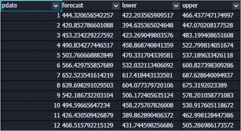
    -DoutputDetailTableName=pai_ft_x13_arima_out_detail

Output tables

outputPredictTableName — forecast results

Column	Description
`pdate`	Forecast date.
`forecast`	Predicted value.
`lower`	Lower bound of the confidence interval (default: 95%).
`upper`	Upper bound of the confidence interval (default: 95%).

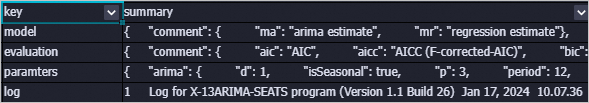
outputDetailTableName — model details

Column	Description
`key`	Record type: `model` (model specification), `evaluation` (evaluation metrics), `parameters` (training parameters), or `log` (training logs).
`summary`	Detail content for the corresponding key.

FAQ

Why are all prediction results the same value?

The model fell back to a mean model, which outputs the training data mean for all forecast steps. This happens when training fails due to instability after temporal differencing, non-convergence, or zero variance. To see the exact error, open the Logview for the job and check the stderr file for individual nodes.

How do I choose p, d, q, sp, sd, and sq values?

If you are not confident in the parameter settings, use x13_auto_arima instead. Set only the upper limits for each order, and x13_auto_arima searches for the optimal values automatically.

Error: `Number of observations after differencing and/or conditional AR estimation is 9, which is less than the minimum series length required for the model estimated, 24`

The training data is too short for the specified model. Modify the frequency parameter or add more historical data.

Error: `Order of the MA operator is too large`

In most cases, this error occurs because the training data is insufficient. Add more training data.

Error: `Series to be modelled and/or seasonally adjusted must have at least 3 complete years of data`

When you specify seasonal parameters (seasonal), the input must contain at least three complete years of data.

What's next

x13_auto_arima — automatically selects SARIMA orders within upper bounds you specify
SQL Script — run PAI commands in a pipeline
MaxCompute client (odpscmd) — upload data to MaxCompute tables