What Is a Relational Model?
Introduction to the Relational Model
Quick BI’s relational model is a data modeling framework designed for multi-table association and analysis. It addresses common challenges in traditional physical modeling—such as low efficiency, insufficient accuracy, and limited analytical flexibility—and supports multidimensional analysis in complex business scenarios.
In the relational model, you do not need to manage data details or specify explicit join types. Simply place related tables on the canvas and configure their join keys to complete modeling easily.
The relational model significantly improves modeling efficiency while ensuring data correctness. Quick BI dynamically adjusts the query SQL based on the fields used in a query and your relationship configuration to guarantee accuracy. For details about how this works, see How Does the Relational Model Work?
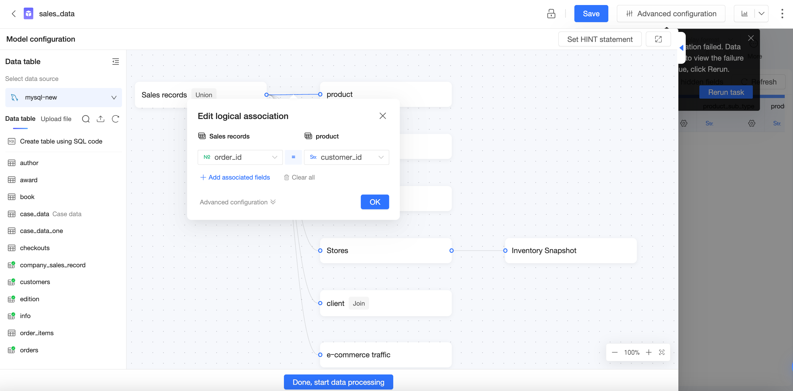
Core Value of the Relational Model
Background and Pain Points
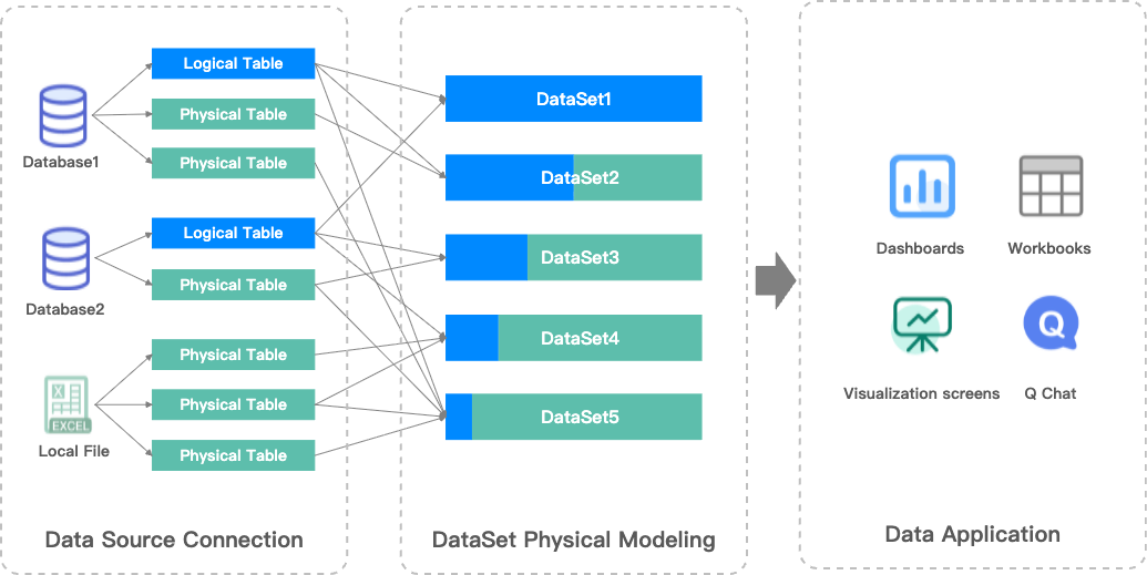
In earlier versions of Quick BI, datasets were modeled using standard physical joins—such as Left Join or Full Join—which produced a single large wide table after joining. Because physical joins can cause data bloat, users typically needed a clear understanding of their data beforehand—including data integrity and uniqueness—to ensure correctness. In some cases, users even had to preprocess source tables, such as by pre-aggregating data, to avoid data bloat. As a result, physical modeling often involved high barriers to entry, significant operational overhead, and a risk of data errors due to data bloat.
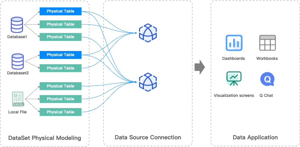
To solve these issues, Quick BI introduced the new relational model, which adds relationship-based modeling capabilities on top of physical modeling. This approach greatly improves efficiency and flexibility when working with complex data models.
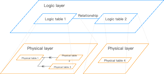
Value of the Relational Model
Simpler data modeling: You only need to specify join fields—no need to choose join types. The relational model handles the rest automatically to ensure data integrity.
Eliminates data bloat: When data granularities do not match, you no longer need to preprocess data during modeling. The relational model resolves data bloat automatically and ensures accurate calculations.
Supports more analytical scenarios without repeated modeling: The relational model is highly reusable. You do not need to build separate models for each analytical scenario, which reduces the total number of models and simplifies maintenance and management.
For more information, see the advantages of the relational model.
Comparison Between Physical and Relational Models
Physical Model | Relational Model |
|
|
Problems:
| Solutions:
|
Key Concepts
Fact Tables and Dimension Tables
Fact tables and dimension tables are common terms in data modeling that describe two different types of tables.
Fact table: Stores quantifiable business metrics containing facts related to a business process. Examples include course completion counts, quiz average scores, and learning duration in an online education platform.
Dimension table: Stores descriptive attributes containing dimensions related to a business process. Examples include course type, student grade level, instructor name, and learning date.
Fact and dimension tables are linked through shared fields. This lets you associate dimensions with metrics during queries and analysis, enabling multidimensional analysis.
Example
Fact Tables
Order Table
Order ID | Date | Product ID | Quantity | Amount |
1 | 2025-12-01 | A | 1 | 50 |
2 | 2025-12-01 | A | 2 | 100 |
3 | 2025-12-01 | B | 3 | 60 |
4 | 2025-12-02 | C | 1 | 10 |
Inventory Records
Date | Product ID | Inventory Quantity |
2025-12-01 | A | 10 |
2025-12-01 | B | 20 |
2025-12-01 | C | 5 |
2025-12-02 | C | 4 |
Dimension Table
Product ID | Product Name | Category | Brand |
A | Vinda Facial Tissues (One Carton) | Household Goods | Qingfeng |
B | M&G File Folders (One Set) | Stationery | Morning Light |
C | Prawn Crackers by Oishi (Large Pack) | Food | Oishi |
Layers in Data Modeling
Each dataset you create in Quick BI has a data model. Think of this model as a relationship diagram of data tables that tells Quick BI how to query your database tables.
Logical Layer and Physical Layer
Quick BI’s data model has two layers:
Logical layer:
When you open the dataset modeling canvas, you first see the logical layer. In most cases, you only need to model at this layer.
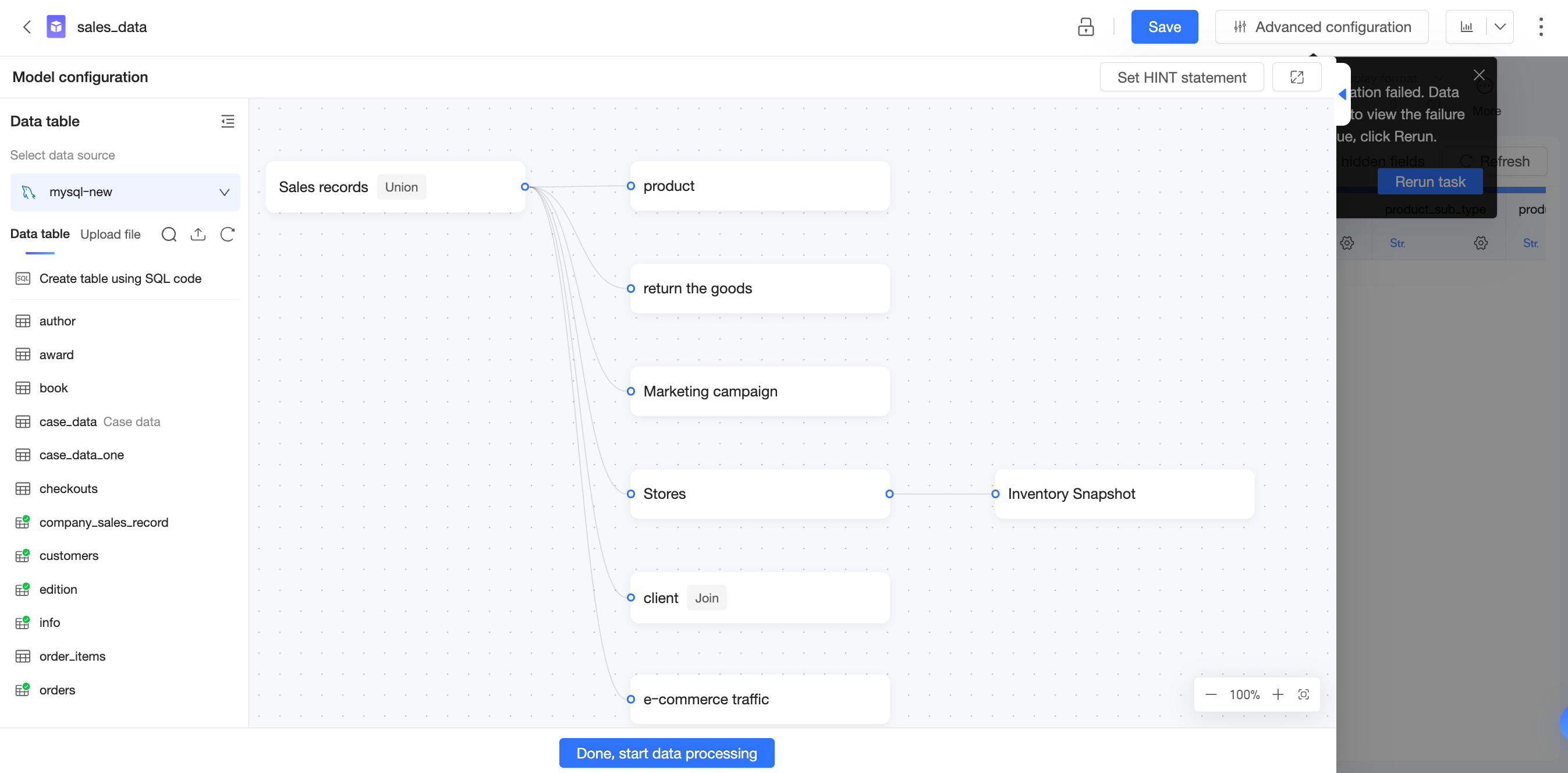
Use relationships—relationship lines—to define connections between nodes. Each node represents a logical table, which can be a single table, a custom SQL statement, or a wide table formed by physically joining or merging multiple tables or SQL statements.
Modeling at the logical layer constructs the complete data model.
Physical layer:
From any logical table in the logical layer, you can access its physical canvas—the physical layer.
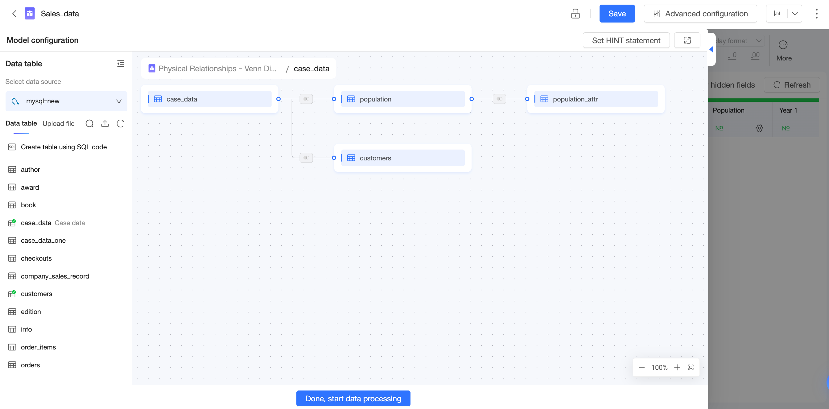
The physical layer uses traditional physical joins or merges to define relationships among physical tables. Each node is either a database table or a custom SQL statement.
Modeling at the physical layer produces a fixed wide table, which becomes a single logical node in the logical layer.
Logical Layer | Physical Layer |
Relationship lines | Venn diagrams |
|
|
Relationship Between Logical and Physical Layers
In the logical layer, logical tables are connected through relationships to form a relational model. You do not need to specify a join type for these relationships, and no fixed wide table is created.
Each logical table corresponds to a separate physical model—either single-table or multi-table—in the physical layer. Double-click a logical table or use the  icon → “Enter Physical Canvas” to access its physical layer. In the physical layer, you must specify exact join types when modeling relationships via joins or merges, and the result is a fixed wide table.
Each logical table in the logical layer has a corresponding physical model—either single-table or multi-table—in the physical layer.
In earlier Quick BI versions, data models had only a physical layer. Starting with V6.1, models include both logical and physical layers, adding support for the relational model.
Relationship Type and Data Match Degree
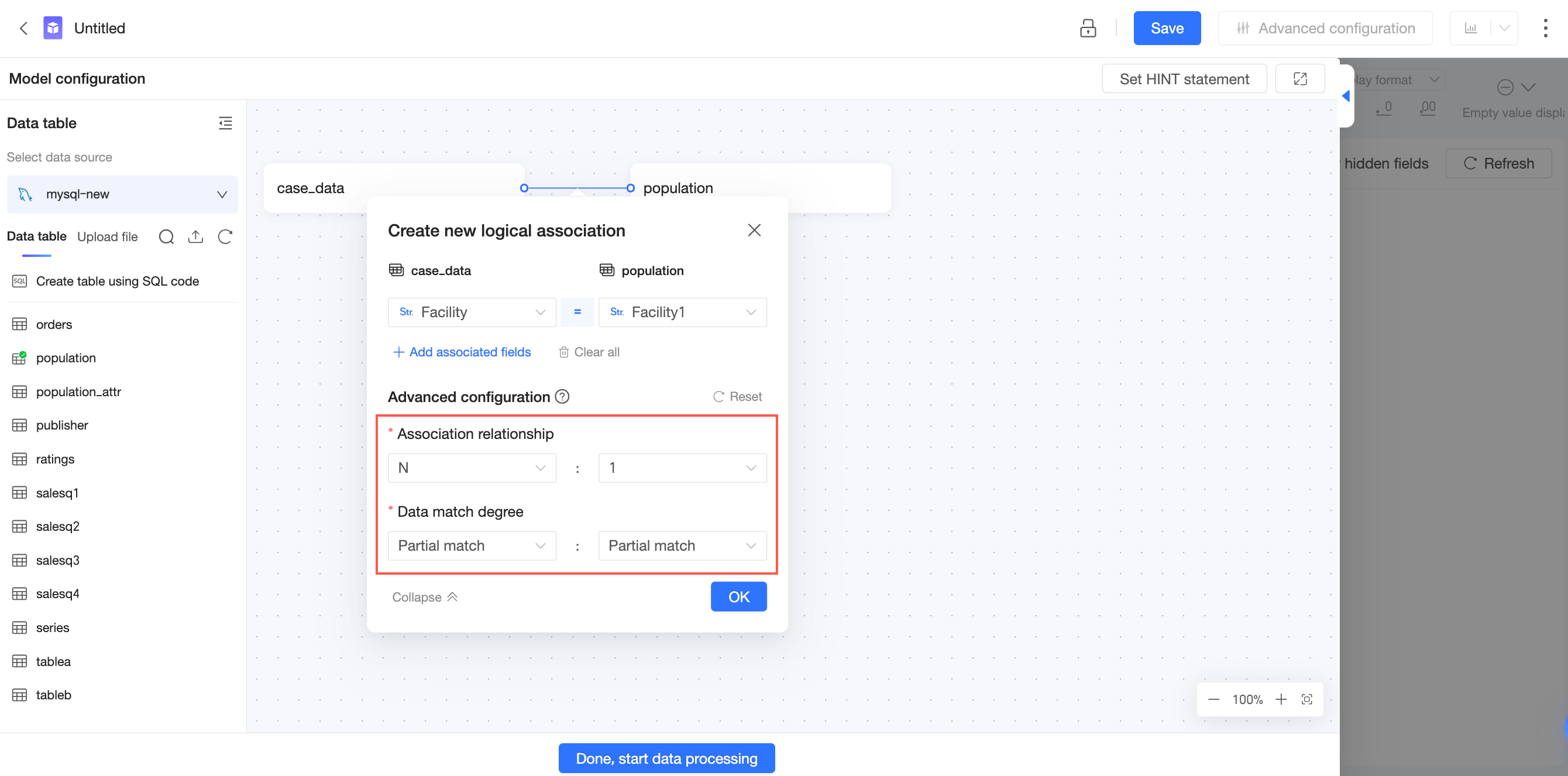
When configuring a relationship, click “More Options” to set the relationship type and data match degree. Quick BI uses these settings to select the optimal join method for queries. Accurate configuration improves query performance.
If you are unfamiliar with your data distribution or the concepts of relationship type and data match degree, keep the default settings. Changing them incorrectly may cause data bloat or data loss.
Only adjust these settings if you fully understand your data distribution and are confident it will not change in the future. This can optimize query performance in the relational model.
Association
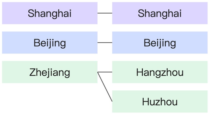
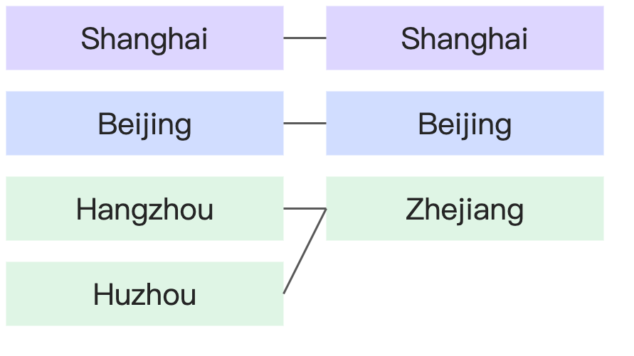
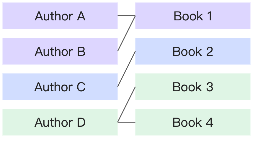
Relationship type indicates whether join key values in one table are unique and whether values in both tables correspond uniquely.
1: Values are unique.
N: Values are not unique.
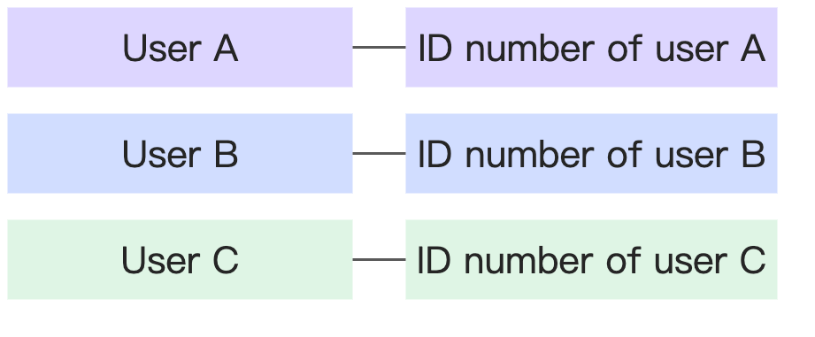
Relationship Type | Example | Diagram |
1:1 | Each person has exactly one ID number, and each ID number belongs to exactly one person. |
|
1:N | Each province has many cities, but each city belongs to only one province. |
|
N:1 |
| |
N:N | One book can have multiple authors, and one author can write multiple books. |
|
Data Match Degree
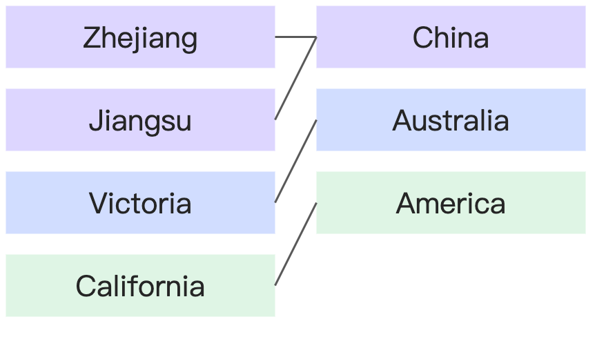
Data match degree indicates whether all join key values in one table can be fully matched to the other table—that is, whether the data is complete.
Partial match: Some values cannot be matched to the other table.
Exact match: All values can be matched to the other table.
Data Match Degree | Example | Diagram |
Match All | Every country has provinces, and every province belongs to a country. |
|
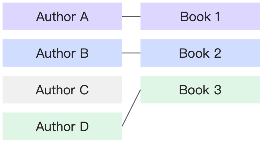
Partial match: full match | Every book has an author, but some authors may not have published books yet. |
|
Exact: Partial | ||
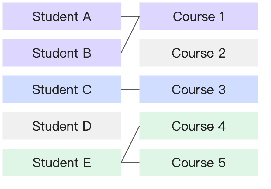
Match type: Partial match | Some students haven’t enrolled in courses, and some courses have no enrolled students. |
|
Scenarios for Using the Relational Model
Applicable Scenarios
Scenario 1: Simple Data Modeling for Business Users
Use the relational model if you have limited knowledge of SQL or databases.
Relational modeling is simpler than physical modeling. Just specify join keys between tables and keep advanced settings at their defaults. The relational model prevents data bloat automatically and eliminates the need to manage data integrity or uniqueness, lowering the modeling barrier and improving accuracy.
Example
An HR department implements a points system to encourage employees to attend training and events. Employees earn points for participation and redeem them for gifts. The underlying database has two tables:
Points Earned Table: Date, Employee ID, Department, Activity Name, Points Earned
Points Redeemed Table: Date, Employee ID, Department, Gift Name, Points Redeemed
These tables have the following relationship:
Points Earned Table – Points Redeemed Table | ||
Relationship Type | N:N | An employee can participate in multiple activities and redeem gifts multiple times. “Employee ID” is non-unique in both tables. |
Data Match Degree | Scope: All | Xiao Wang has earned points but has never redeemed gifts, so Xiao Wang appears in the Points Acquisition Table but not in the Points Redemption Table; If an employee has never earned points, they cannot redeem gifts. Consequently, the Points Redemption Table cannot have an entry if the Points Acquisition Table does not. |
HR wants to analyze each employee’s remaining points. A naive approach would join the tables directly on Employee ID. But because Employee ID is non-unique in both tables, this causes data bloat. The correct physical modeling approach requires pre-aggregating both tables by Employee ID before joining—a task requiring data preprocessing skills.
With the relational model, HR simply joins on Employee ID. Quick BI automatically handles aggregation during calculation to ensure correctness.
For more details, see How Does the Relational Model Work?
Scenario 2: Improved Dataset Reusability Across Multiple Analytical Scenarios
When many underlying tables exist, IT teams can drag all related tables into the logical canvas to build a single comprehensive relational model. Business users then select only the fields they need. This avoids creating separate wide tables for each analytical scenario, preventing dataset proliferation and simplifying maintenance.
In this scenario, IT should accurately configure relationship type and data match degree based on data characteristics to improve query performance and reduce the impact of complex modeling.
Example
Consider the same HR points scenario:
Points Earned Table: Date, Employee ID, Department, Activity Name, Points Earned
Points Redeemed Table: Date, Employee ID, Department, Gift Name, Points Redeemed
Unlike the previous example, a centralized IT team must prepare datasets for all analysts. HR requests support for three scenarios. With physical modeling, IT would need to build three separate datasets.
Scenario | Analysis Description | Physical Modeling Approach |
Scenario 1 | Analyze participation count and points earned per activity | Points Earned Table (single-table model) |
Scenario 2 | Analyze redemption count and participant count per gift | Points Redeemed Table (single-table model) |
Scenario 3 | Analyze each employee’s remaining points and show a leaderboard | Aggregate both tables by “Employee ID,” then join |
Because the two tables have different granularities, a direct physical join causes data bloat and incorrect results. But aggregating by Employee ID loses details such as Activity Name and Gift Name, making Scenarios 1 and 2 impossible. Thus, physical modeling requires three separate datasets.
With the relational model, IT builds just one dataset. Quick BI automatically selects the right calculation method based on the fields used in each analysis to ensure correctness.
Scenario | Analysis Description | Relational Modeling Configuration | Drag into Field | Relational Model Handling |
Scenario 1 | Analyze participation count and points earned per activity | Join Key: Employee ID N:N Section: All | Dimension: Activity Name Measure: Employee ID (distinct count), Points Earned (sum) | Single-table query |
Scenario 2 | Analyze redemption count and participant count per gift | Dimension: Gift Name Measure: Employee ID (distinct count), Points Redeemed (sum) | Single-table query | |
Scenario 3 | Analyze each employee’s remaining points and show a leaderboard | Dimension: Employee ID Measure: SUM(Points Earned) - SUM(Points Redeemed) | Aggregated join |
For more details, see How Does the Relational Model Work?
Limits of the Relational Model
Performance Limits
To prevent data bloat, the relational model applies special processing to query SQL, making it more complex. Compared to traditional physical joins, queries generated by the relational model contain more subqueries and nesting levels, which can reduce performance. Performance also depends heavily on data volume and model complexity. As these increase, the performance gap between relational and physical models widens.
If you understand your data distribution well, you can optimize query performance by adjusting relationship type and data match degree. Generally, performance ranks as follows:
Relationship type: 1:1 > 1:N = N:1 > N:N
Data match degree: Exact:Exact > Exact:Partial = Partial:Exact > Partial:Partial
If you are unfamiliar with your data distribution or the concepts of relationship type and data match degree, keep the default settings. Changing them incorrectly may cause data bloat or data loss.
Only adjust these settings if you fully understand your data distribution and are confident it will not change in the future. This can optimize query performance in the relational model.
Even so, if you have strong data processing skills and require very high query performance, we recommend continuing to use traditional physical modeling to avoid the extra computation introduced by the relational model’s complex logic.
Data Volume Limit
When measures come from multiple logical tables, Quick BI queries and calculates each logical table separately, then joins the results. To ensure query efficiency and service stability, each query is limited to 10,000 rows. For details, see How Does the Relational Model Work?
This 10,000-row limit applies to aggregated results. For example, if the join field is Region and the query dimension is Product Type, Quick BI aggregates by Region and Product Type and returns up to the first 10,000 rows.
Due to the computational complexity of the relational model, you cannot paginate beyond 10,000 rows. If your query dimensions have many enumeration values or if you require more detailed granularity, the relational model may return incomplete results. In such cases, we recommend using traditional physical joins for modeling.
Feature Limits
The introduction of the relational model required significant changes to dataset processing and computation. The following features are incompatible with older versions:
Resource plans cannot import datasets from newer versions into older environments. Upgrade your target environment to V6.1 or later before importing resource plans.
The legacy dataset detail query API QueryDatasetDetailInfo no longer supports relational model datasets. Switch to the new API: QueryDatasetInfo.
Legacy API (no longer maintained): https://next.api.aliyun.com/document/quickbi-public/2022-01-01/QueryDatasetDetailInfo
New API: https://next.api.aliyun.com/document/quickbi-public/2022-01-01/QueryDatasetInfo
Quick BI introduced the initial version of the relational model in V6.1. The following features currently support only single-logical-table datasets. Support for multi-logical-table datasets will be added in future versions:
Data Preparation
Complex filter conditions cannot use fields from multiple logical tables. The following features are affected:
Row-level permissions, including conditional combination authorization and user tag–based authorization
Dashboard composite query controls
Monitoring and Alerts alert rules
Extraction acceleration limit: If a query involves more than three logical tables, the system bypasses the acceleration engine and executes the query directly via live connection.