Create intelligent inspection task for unlabeled data

Sample data

This topic uses sample data to demonstrate how to create a model training job and a real-time inspection task. The data is stored in the operation-metric Logstore and contains fields such as Region, Method, and Latency.

Step 1: Create a model training job

1. Log on to the Simple Log Service console.

2. Navigate to the job creation page.

   1. In the Log Application section, on the Intelligent O&M tab, click Intelligent Anomaly Analysis.

   2. In the Instance List, click the target instance.

   3. In the left-side navigation pane, choose Analysis Jobs > Intelligent Inspection > Model Training.

   4. In the Model Training Jobs section, click Create Now.

3. In the Create Model Training Job wizard, on the Basic Information step, configure the following parameters, select the region where the source Logstore is located, and then click Next.

   Parameter	Description
   Task name	The name of the model training job.
   Project	Select the Project where the source Logstore is located.
   Logstore type	The location where the source data is stored. In this example, select Logstore.
   Source logstore	Select the Logstore where the source data is located.
   Role	If you granted permissions when you created the instance, the AliyunLogETLRole identifier is automatically displayed.
   Destination logstore	The destination Logstore. This parameter is fixed to internal-ml-log.

4. In the Create Model Training Job wizard, on the Data feature configuration step, configure the following parameters.

   1. On the Data feature configuration tab, configure the following parameters.

      Because this example's data has no anomaly labels, you must first use anomaly injection to generate them.

      Important

      You must include a LIMIT clause in your SQL statement to prevent incomplete data extraction.

      For Data type, select Format data with SQL and enter an SQL query to extract the required fields. In this example, set Time to time, Granularity to 60 seconds, Entity to Region and Method, and Feature to Latency. For Anomaly injection, select Do not save, and set Anomaly rate to 0.001.

      Parameter	Description
      Time	The field in the source data that identifies the time column.
      Granularity	The observation interval of the data. Unit: seconds. Valid values: 5 to 3600.
      Entity	The fields in the source data that identify the specific entity.
      Feature	The field in the source data that identifies the feature value.
      Anomaly injection	Specify whether to save the injected anomaly data. Save: Saves the injected anomaly data to a Logstore named <SourceLogstoreName>_withlabel in the same Project as the source data. For example, if the source data is in the sls-test-demo Project and the sls-test-logstore Logstore, the injected anomaly data is saved to the sls-test-logstore_withlabel Logstore within the sls-test-demo Project. Do not save: Does not save the injected anomaly data.
      Anomaly rate	The proportion of injected anomalies relative to the total amount of data. Valid values range from 0.00001 to 0.01. The injected anomalies are randomly and evenly distributed across the dataset.
      Anomaly type	Anomaly types include extreme value anomalies, trend anomalies, drift anomalies, and variance anomalies. For more information, see Anomaly types.

5. In the Create Model Training Job wizard, on the Algorithm configuration step, configure the following parameters and then click Finish.

   Currently, only the supervised anomaly detection algorithm is supported. The page also includes an optional Single-dimension feature configuration section that you can configure as needed.

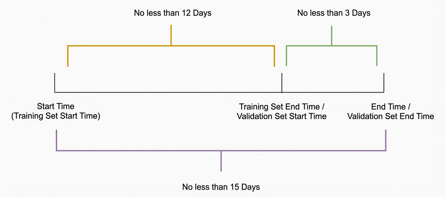
   The time configuration includes the training start time (start of the training set), training end time (start of the validation set), and validation end time (end of the validation set). The relationship between these times is shown in the following figure.

Step 2: View the training results

After the job has run for a period, you can view the training results by clicking the job in the model training job list. For a detailed description of the training results, see intelligent inspection (model training).

View job information

On the Model Training Job Details page, you can view the stages of the job execution: Read Training Data > Training Data Read Complete > Start Model Training > Model Training Complete > Read Validation Data > Validation Data Read Complete > Start Predicting Validation Data > Prediction Complete, Generating Report > Start Saving Model > Model Saved > Job Complete. The total time for the job is also displayed.

View entity information

In the Entity Information List, click an entity and then click View task details of the entity. The details page includes the following:

• The Single Entity Progress chart shows the entity's progress through the following stages: Start Feature Engineering > Feature Engineering Complete > Start Model Training > Model Training Complete > Start Training Prediction > Training Prediction Complete > Start Validation Prediction > Validation Prediction Complete > Generating Report > Report Generation Complete. The start and end times of each stage are displayed on a timeline.

• The Time configuration chart displays time-related information for model training. This includes Training Start Time, Training End Time, Validation End Time, Model Training Duration, and Model Validation Duration.

• The Validation set evaluation metrics chart displays the auc, macro_f1, precision, and recall metrics. In this example, auc is 0.7494, macro_f1 is 0.7988, precision is 0.8733, and recall is 0.7494.

  Metric	Description
  auc	The Area Under the Curve (AUC), where the curve is plotted with the true positive rate against the false positive rate. The false positive rate is the number of normal samples identified as anomalous divided by the total number of normal samples. The true positive rate is the number of anomalous samples identified as anomalous divided by the total number of actual anomalous samples. This is equivalent to recall.
  macro_f1	The harmonic mean of precision and recall. Formula: F1 = 2 * (precision * recall) / (precision + recall). This uses the macro-average method, which gives each class equal weight when computing the mean. The final result is the arithmetic mean of the metrics for each class.
  precision	The precision is the number of samples correctly detected as anomalous divided by the total number of samples detected as anomalous.
  recall	The recall is the number of samples correctly detected as anomalous divided by the total number of actual anomalous samples.

• The Data statistics chart shows the length of the training and validation sets, and the number of anomalous points in each.

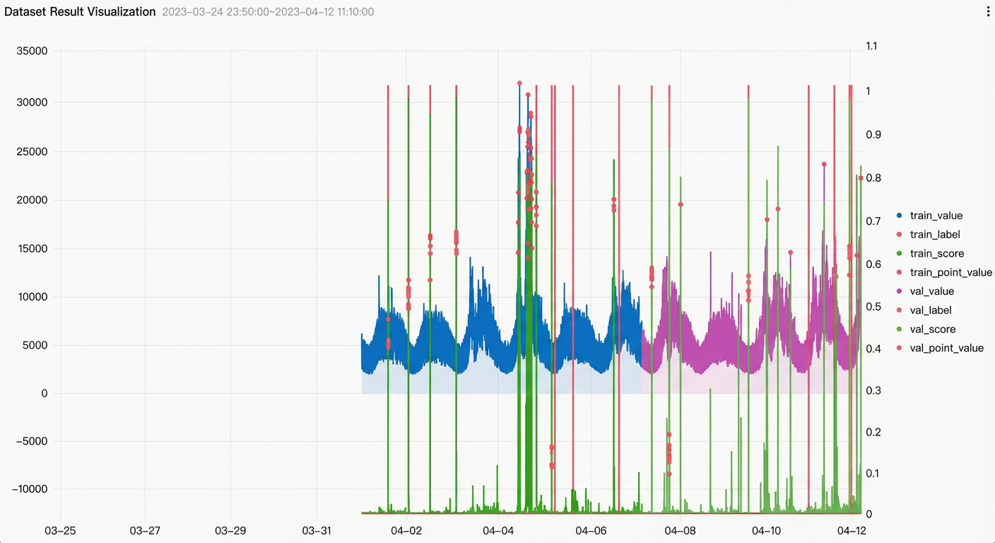
• The Dataset result visualization chart visualizes the changes in the training and validation sets. You can drag the chart to view the curve in more detail.

  The blue area represents the training set, and the red area represents the validation set. The red vertical lines indicate actual, labeled anomalies. The green curve represents the predicted anomaly score.

  Points on the data curve are marked in red if their predicted anomaly score exceeds the threshold defined in the Anomaly score text box. By default, the threshold is 0.5.

  Field	Description
  train_value	The value of a feature in the training set.
  train_label	The anomaly label for the training set.
  train_score	The predicted anomaly score for the training set.
  train_point_value	Equivalent to train_value. This field is used to mark anomaly points in the chart. When the predicted anomaly score for the training set is greater than the threshold, the point corresponding to train_point_value is marked in red. By default, the threshold is 0.5. You can set the anomaly score threshold in the Anomaly score text box on this page.
  val_value	The value of a feature in the validation set.
  val_label	The anomaly label for the validation set.
  val_score	The predicted anomaly score for the validation set.
  val_point_value	Equivalent to val_value. This field is used to mark anomaly points in the chart. When the predicted anomaly score for the validation set is greater than the threshold, the point corresponding to val_point_value is marked in red. By default, the threshold is 0.5. You can set the anomaly score threshold in the Anomaly score text box on this page.

• The Anomaly event list table shows detailed information about anomaly events. The list includes columns such as anomaly_time (time of anomaly), entity, dim_name (dimension name), value (feature value), score (anomaly score), and anomaly_type.

Step 3: Create a prediction task

1. On the model training job details page, click Create Prediction Task in the upper-right corner.

2. In the Create Prediction Task panel, configure the following parameters and click OK. You can also use the Enable smart merge switch at the bottom of the panel.

   Parameter	Description
   Task name	The name of the prediction task.
   Entity ID	Select the entity for real-time inspection.
   Start time	Corresponds to the end time of the model training job and cannot be changed.
   Data latency	Set the data latency based on your data write delay. For example, if your data is written to the Logstore with a 60-second delay, set this value to at least 60 seconds.
   Generate alert	Select Yes to configure alerting on inspection results.
   Alerting policy	An alerting policy merges, silences, and suppresses generated alerts. If you select simple mode or normal mode, you do not need to configure an alerting policy. Log Service uses the built-in dynamic alerting policy (sls.builtin.dynamic) for alert management by default. If you select advanced mode, you can select a built-in or custom alerting policy for alert management. For more information about how to create an alerting policy, see Create an alerting policy.
   Action policy	An action policy controls the alert notification channels and their frequency. If you set Alerting Policy to simple mode, you only need to configure an action group. After you configure the action group, Log Service automatically creates an action policy named RuleName-ActionPolicy. All alerts triggered by this alert rule are sent by using this action policy. For more information about the configuration, see Notification methods. Important You can modify this action policy on the Action Policy management page. For more information, see Create an action policy. If you add conditions when you modify the action policy, the Alerting Policy automatically changes to normal mode. If you set Alerting Policy to normal mode or advanced mode, you can select a built-in or custom action policy for alert notifications. For more information about how to create an action policy, see Create an action policy. If you set Alerting Policy to advanced mode, you can also enable or disable Custom action policy. For more information, see Dynamic action policy mechanism.

Step 4: View the inspection results

After you create an inspection task, click the task in the real-time inspection task list to view its details. For a detailed description of the inspection results, see intelligent inspection (real-time monitoring). The details page displays statistical information about the inspection job, including the Number of Inspection Metrics, Number of Extreme Metrics, entity consumption progress, entity metric list, and an observed value time-series chart.