Asight Compute GUI

Once you generate a.acurep report on the target using the acu command-line tool, you can copy it to the host and open it with the Asight Compute GUI.

UI Feature Highlights

• Configure various performance metrics to display data in multiple formats, such as tables and charts.

• View the detailed memory workload hierarchy as both a diagram and a table.

• Use the baseline feature to compare performance results across different kernels and reports to identify differences.

• From the Raw Page, you can export reports as PDF, PNG, or CSV files. You can also export the raw report data as a CSV file for further analysis.

• Use the project explorer to manage reports, which lets you open and delete selected reports in bulk.

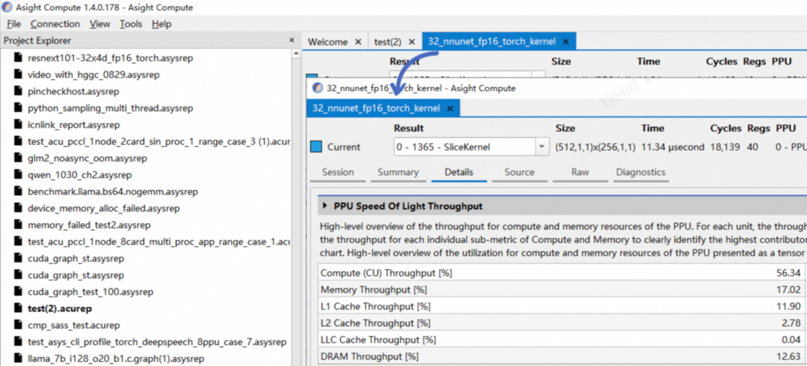
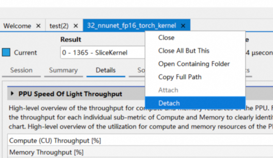
• The dock widget lets you drag reports out of the main window, so you can view them in separate windows or on different screens, as shown below.

You can dock a window by dragging and dropping its tab:

You can also use the Detach or Attach option in the context menu:

1. Details

The details page presents all metrics collected during kernel startup. It is divided into sections. Each section includes a header table showing the key metrics for that topic. Most sections also include at least one expandable and collapsible section body, presenting more detailed metrics in tables or charts, as shown in the figure below:

1. Expand or collapse section body

2. Section description

3. Header table

4. Switch section body

5. Section body

Hover over a table or chart to see exact metric values, detailed information, and term definitions, as shown below.

The sections below list potential kernel bottlenecks and provide optimization suggestions:

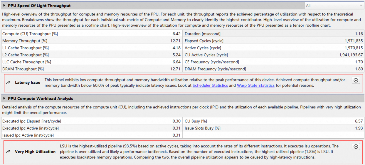
Besides the built-in rules, Asight Compute lets you create custom rules by modifying .py files. See rule system for details.

The details page is broken down into sections covering compute load, cache hit, and Warp scheduling. Analyze these metrics to understand the kernel's runtime behavior and identify bottlenecks and opportunities for optimization.

Each section is described below.

1.1 Speed-of-light throughput

This section provides an overview of the PPU's compute and memory resource utilization during kernel execution. It shows kernel throughput as a percentage of its theoretical peak for both computation and memory access. This is the typical starting point for analysis to determine if a kernel's performance is compute-bound or memory-bound.

1.1.1 Header table

The header table provides an overview of PPU unit throughput utilization and the number of kernel execution cycles:

1.1.2 PPU throughput bar chart

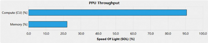
This bar chart shows the throughput percentages for compute and memory units. These categories correspond to the table headers Compute (CU) Throughput and Memory Throughput.

This chart shows whether a kernel's performance is limited by compute or memory access, helping you choose the right optimization strategy. Kernels are typically classified into the following three types based on their performance bottleneck:

Compute-bound kernel

A kernel is considered compute-bound when it pushes the throughput of a PPU compute unit near its theoretical maximum (typically over 80%), as shown in the figure below.

A kernel is compute-bound when its compute instructions greatly outnumber its memory accesses. To improve performance further, check the Compute Workload Analysis section to find the most utilized compute unit pipeline:

• Consider converting this type of computation to a different one.

• Eliminate redundant computations to reduce the workload.

• Use a lookup table instead of computation.

Memory-bound kernel

When a kernel drives the throughput of a PPU memory unit near its theoretical maximum (typically over 80%), the kernel's performance is limited by memory access. Such a kernel is called memory-bound, as illustrated in the figure below.

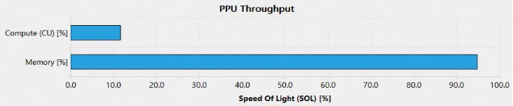
A memory-bound kernel spends most of its runtime waiting for data. To improve performance, refer to the Memory Workload Analysis section for guidance on optimizing your memory subsystems:

• Ensure coalesced access to global memory.

• Maximize use of the memory hierarchy, such as shared memory and caches.

• Maximize data reuse to reduce memory access instructions.

• Use on-the-fly computation instead of lookup tables.

latency-constrained kernel

A kernel is considered latency-bound when it can't achieve its theoretical peak performance for either computation or memory access, as illustrated in the figure below.

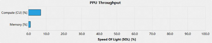
For a latency-limited kernel, check the Launch Statistics section to verify the launch configuration and ensure the grid is large enough. Review the Scheduler Statistics and Warp State Statistics sections to determine why threads wait instead of executing.

To optimize a latency-bound kernel:

• Use enough blocks to fill the PPU and maximize occupancy.

• Increase the workload per thread, for example, by having each thread process multiple input elements.

1.1.3 Breakdown tables

The two types of Breakdown Tables show the throughput percentages for individual PPU computing and memory units, as shown below:

The breakdown table helps you identify which unit is limiting the kernel by listing the throughput percentage of each unit in descending order. The bar chart then displays the throughput of the busiest unit, which is treated as the throughput of the entire subsystem.

1.1.4 Roofline Chart

A kernel requires data to compute. Therefore, its performance depends on both the PPU's computing speed and the speed at which data is supplied to the kernel. To visualize kernel performance, Asight Compute provides a roofline chart. This chart combines the PPU's peak computing performance and memory bandwidth with a metric called arithmetic intensity—the ratio of work to memory traffic. A typical roofline chart is shown in the figure below:

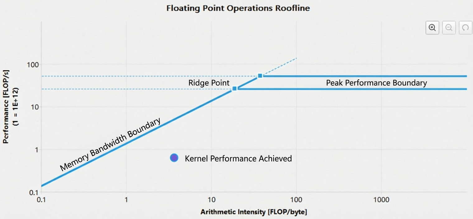
• The y-axis represents floating-point operations per second (FLOPS). Since this value can be very large for a PPU, the axis uses a logarithmic scale to improve visualization.

• The x-axis represents arithmetic intensity, which is the ratio of work (FLOP/s) to memory traffic (bytes/s), measured in FLOP/byte. This axis also uses a logarithmic scale.

• The memory bandwidth boundary, the sloped part of the roofline, is determined by the PPU's memory bandwidth.

• The peak performance boundary, the horizontal part of the roofline, is determined by the PPU's peak computing performance.

• The ridge point is the intersection of the memory bandwidth boundary and the peak performance boundary. This point helps analyze kernel performance.

• The achieved performance point indicates a kernel's performance at its current arithmetic intensity. When performing a baseline comparison, the performance values of the baselines are also displayed. A point's outline color identifies its corresponding baseline.

A roofline chart shows whether a kernel is compute-bound or memory-bound, as illustrated by the figure below.

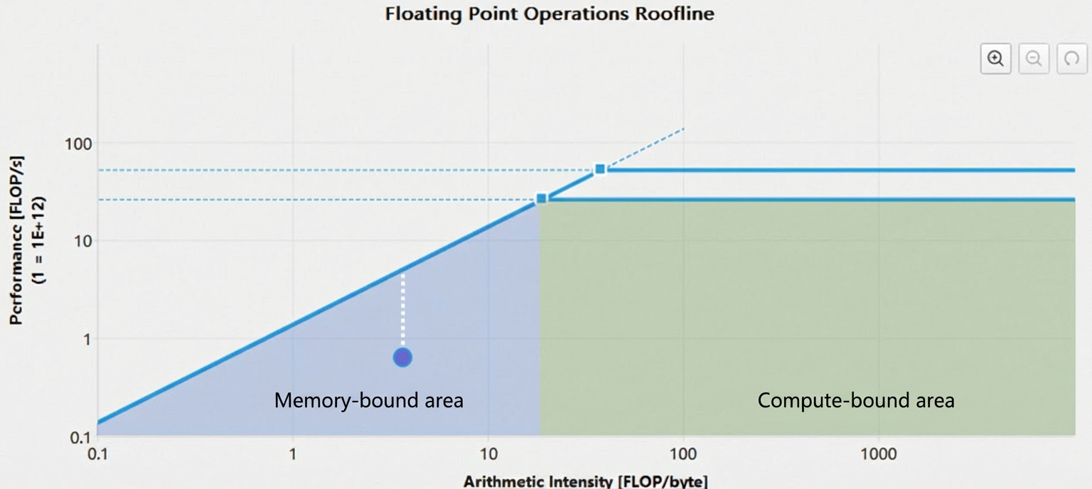
In the figure above, the ridge point divides the roofline into two regions: the memory-bound region (the blue shaded area under the memory bandwidth boundary) and the compute-bound region (the green shaded area under the peak performance boundary). The location of a kernel's achieved performance point determines its primary performance-limiting factor.

The distance from the achieved performance point to the upper bound (represented by the white dashed line in the figure) shows the headroom for performance optimization. The closer the achieved point is to the upper bound, the better the kernel performs. If a kernel is memory bandwidth bound, increasing its arithmetic intensity is the only way to improve performance.

You can zoom and pan the roofline chart for easier viewing:

• Zoom in:

  • Hold Ctrl and scroll up with the scroll wheel.

  • Click and drag with the left mouse button to select an area.

  • Click the zoom in button in the upper-right corner.

  • Press the + key.

• Zoom out:

  • Hold Ctrl and scroll down with the scroll wheel.

  • Click the right mouse button.

  • Click the zoom out button in the upper-right corner.

  • Press the - key.

• Reset:

  • Click the reset button in the upper-right corner.

  • Press the Esc key.

• Pan:

  • Hold Ctrl and drag with the left mouse button.

1.2 Compute workload analysis

The Compute Workload Analysis section provides detailed performance data for the compute resources within the PPU computing unit:

• Instructions per clock (IPC): The number of instructions the CU issues per clock cycle.

• Pipeline utilization: The usage rate of various pipelines in the CU.

1.2.1 Header table

The header table lists key kernel execution metrics, such as CU utilization and the instruction count per active cycle:

1.2.2 Pipe utilization bar chart

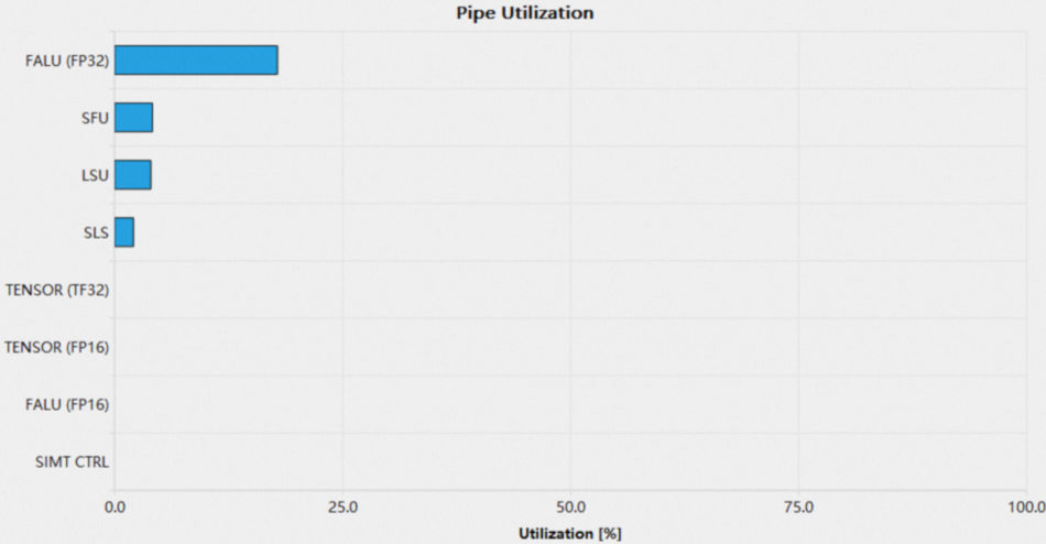
The Pipe Utilization Bar Chart shows the utilization of compute pipes in the PPU during kernel execution. The most common pipelines include:

Low utilization across all compute pipes (typically below 60%) suggests the launch configuration for the kernel is too small or the warp scheduler lacks enough warps to issue. For details, see the Launch Statistics section and the Scheduler Statistics section.

When a pipe's utilization in a compute unit is too high (typically over 80%), it may be a performance bottleneck. To improve performance, consider balancing utilization across all pipes.

1.3 Memory workload analysis

The Memory Workload Analysis section presents detailed performance data for the PPU's various memory units. When these units are heavily used, memory access can become a performance bottleneck for the kernel. A bottleneck occurs when memory unit utilization is too high, memory bandwidth is saturated, or the throughput of memory access instructions reaches its limit. This section contains two subsections:

• Memory chart

• Memory table

1.3.1 Header table

The header table shows utilization metrics for each PPU memory unit, including the cache hit rate, achieved bandwidth, and memory access pipe utilization rate.

1.3.2 Memory chart

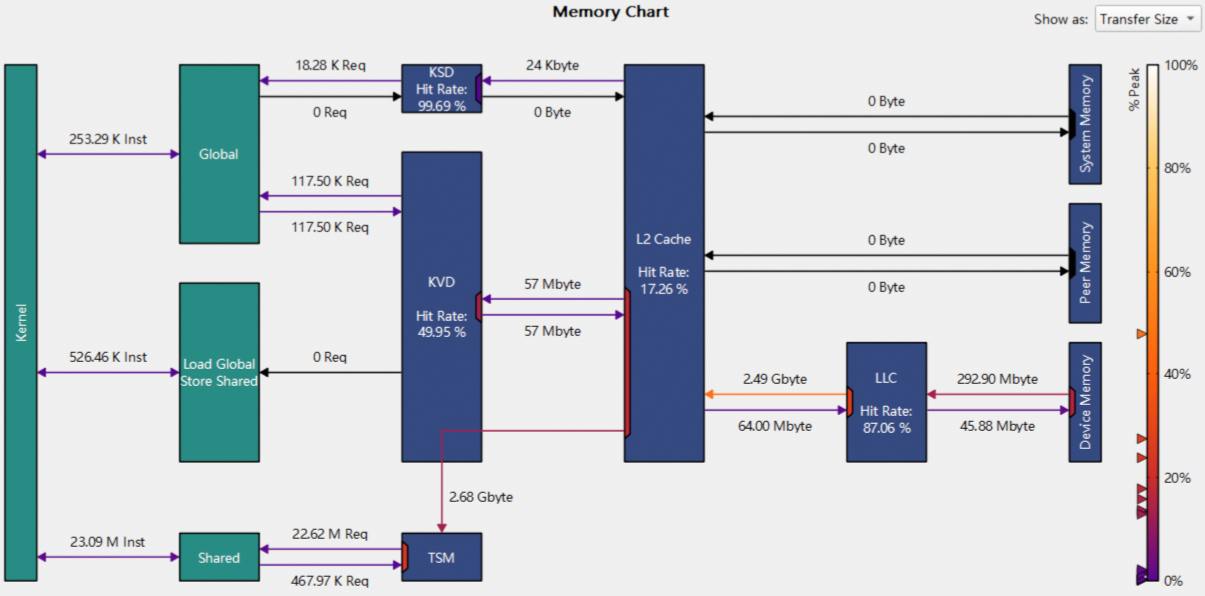
The Memory Chart shows data transfer between memory units, including the cache hit rate, instruction count, and memory request count:

• Logical units (green section), including:

  • Kernel: A kernel running on the PPU.

  • Global: HGGC global memory.

  • Local: HGGC local memory.

  • Shared: HGGC shared memory.

  • Load global store shared: An instruction that loads data directly from global memory to shared memory.

• Physical units (blue section), including:

  • L1 cache: Includes units such as KSD, KVD, and TSM.

  • L2 cache and L2 compression.

  • LLC cache and LLC compression.

  • System memory: system (CPU) memory.

  • Device memory: device (PPU) memory.

  • Peer memory: Memory on other PPU devices.

• Links

  • Links between the Kernel and other logical units represent the number of instructions executed by those units. For example, the link between the Kernel and Global represents the number of global memory load/store instructions.

  • Links between logical units and physical units represent the number of requests issued by the corresponding instructions.

  • Links between physical units represent the amount of data transferred between them.

  • The arrows on the links indicate the direction of data transfer. The color of a link indicates its utilization percentage. The legend on the right shows the colors that correspond to different utilization rates, from 0% to 100%. Some links share a data port. In the chart, colored trapezoids represent data ports, and their color indicates the port's utilization.

• Use the combo box in the upper-right corner to switch between transfer size and throughput.

1.3.3 Memory Table

The memory table shows detailed metrics for various memory units, such as shared memory, cache, and device memory. Hover over an entry to see more details.

1.4 Scheduler statistics

The Scheduler Statistics section details how the warp scheduler performs warp scheduling. Each warp scheduler maintains a warp pool from which it can issue instructions to its warps. The kernel launch configuration limits the size of the warp pool to a maximum of 16 warps. Each cycle, the warp scheduler checks the state of each warp and classifies them into the following four categories:

• Active warp: A warp is active from the time it becomes schedulable by the warp scheduler until it executes its last instruction.

• Eligible warp: A warp that is ready to issue its next instruction, for example, when the data it requires is available.

• Stalled warp: A warp that cannot issue its next instruction because it is waiting for a dependency to be resolved, such as a synchronization barrier or the result of a previous instruction.

• Selected warp: An eligible warp that the warp scheduler has chosen to execute next.

The figure below illustrates the relationships among the warp states:

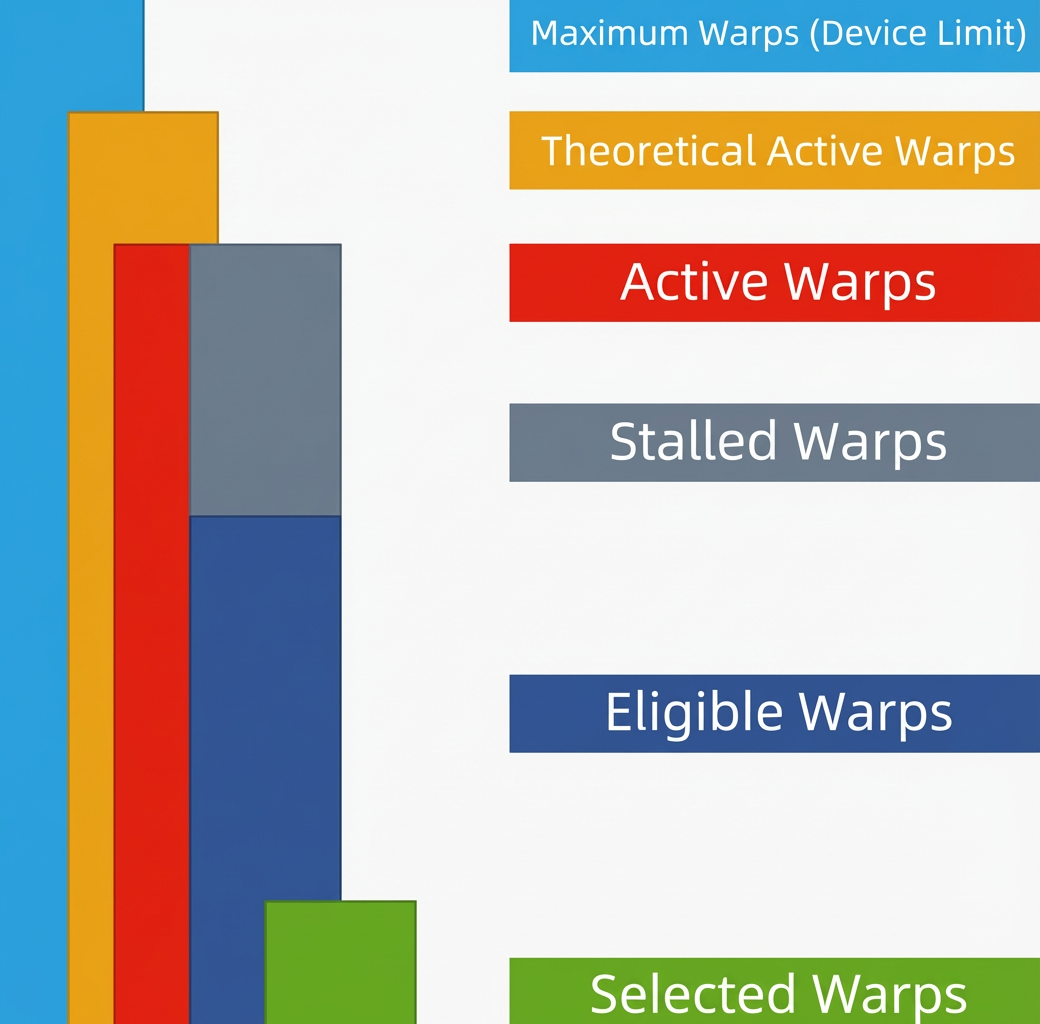
The figure above shows the relationship between Active Warps, Theoretical Active Warps, and the Device Limit: Device Limit >= Theoretical Active Warps >= Active Warps.

An active warp is either a stalled warp or an eligible warp, depending on whether it can issue its next instruction. Thus, active warps = stalled warps + eligible warps.

Each cycle, the warp scheduler selects an eligible warp to issue its next instruction. If no warps are eligible in a given cycle, no instruction is issued, which degrades kernel performance.

1.4.1 Header table

To meet this challenge, we propose a novel approach called Scale-Aware Concurrency Control (SACC). This scheme has two main goals. First, it aims to fully utilize the abundant computing resources on large-scale hardware. Second, it seeks to minimize the performance overhead associated with concurrency control on large-scale hardware, ensuring that the system can efficiently handle a high volume of concurrent transactions without performance degradation.

The header table shows how the warp scheduler issues instructions:

1.4.2 Warps-per-scheduler bar chart

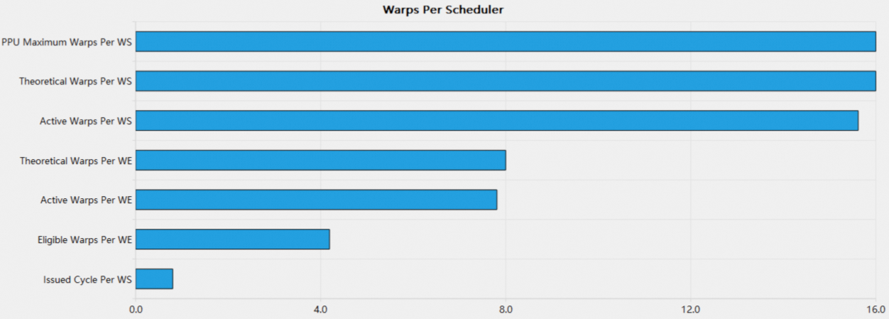
The Warps Per Scheduler bar chart shows the average number of warps per cycle in each state on each warp scheduler.

Ideally, the warp scheduler issues one instruction per cycle. When Issued Warps Per Scheduler is low (typically below 0.6), this indicates that PPU resources are underutilized, degrading kernel performance. An insufficient number of eligible warps is the direct cause of a low Issued Warps Per Scheduler value. To improve kernel performance:

• Review the Occupancy section to ensure high kernel occupancy, aiming for 16 theoretical active warps.

• Review the Warp State Statistics section to identify the primary stall reason, and reduce the associated stall time to increase the number of eligible warps.

• Avoid variations in warp execution time caused by load imbalance.

1.5 Warp state statistics

The Warp State Statistics section shows the average number of cycles a warp spends per instruction during kernel execution. This number determines the latency between instructions. A higher cycle count requires more warp parallelism to hide the latency. The section also provides a breakdown of active warp states during these instruction cycles. A warp state indicates whether a warp is ready to issue its next instruction and the reason for that state.

1.5.1 Warp stall reasons

The PPU defines the following 15 states for active warps:

1.5.2 Header table

The header table contains the following items:

Cycles Per Issued Instruction (CPI) is a key kernel performance metric.

1.5.3 Warps per scheduler bar chart

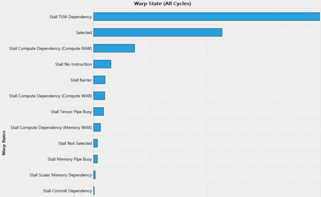
The Warps Per Scheduler bar chart lists all warp stall reasons in descending order. The sum of cycles for all warp stall reasons equals the Warp Cycles Per Issued Instruction. Warp stalls are unavoidable; you should investigate these reasons only when the No Eligible value in the Warp State Statistics section is high.

1.6 Instruction statistics

This section provides statistics on low-level assembly instructions (SASS).

1.6.1 Header table

The header table contains the following items:

1.6.2 Executed instruction mix

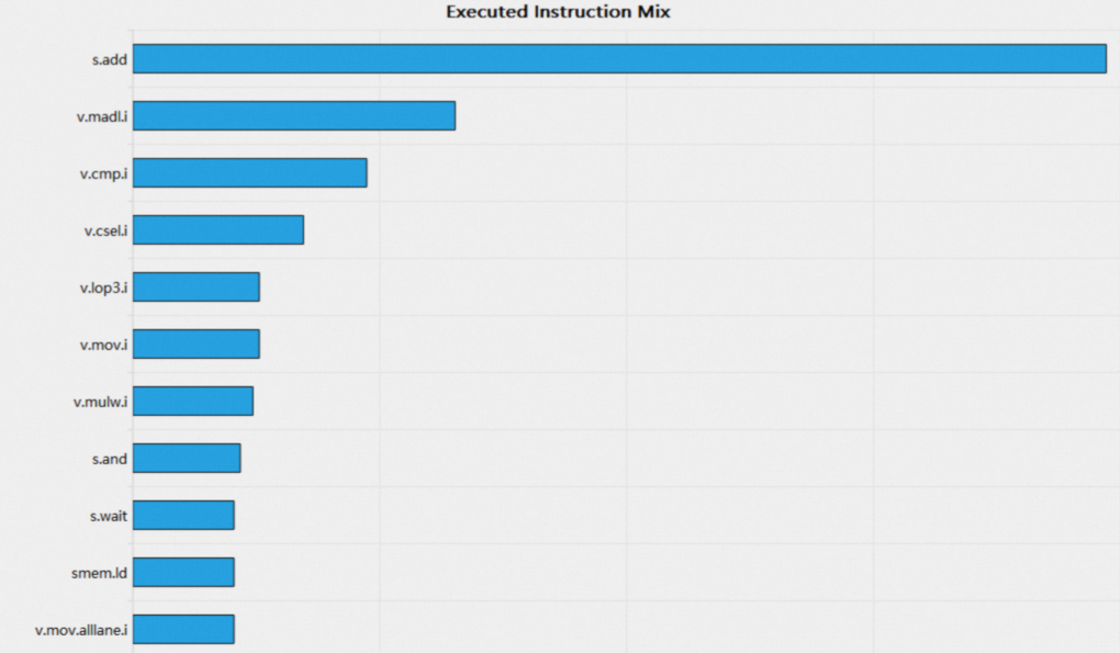
The Executed Instruction Mix bar chart lists all instructions a kernel executes, sorted in descending order by instruction count. Use this chart to identify the ratio of fused instructions, such as fma, to non-fused instructions, such as add and mul. If the ratio of non-fused instructions is high, consider converting them to fused instructions to improve instruction throughput.

1.7 ICNlink

This section provides an overview of ICNlink utilization, including total memory used for sending and receiving, and peak link utilization.

The header table contains the following items:

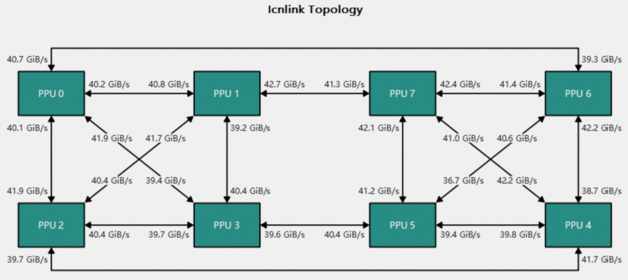
The topology diagram visualizes the connections and data transfer between devices:

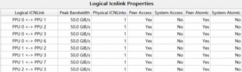
The Attribute Table displays an ICNlink's properties, such as peak bandwidth and the number of physical connections.

This table lists the ICNlink throughput, bandwidth utilization, and idle time for the selected range:

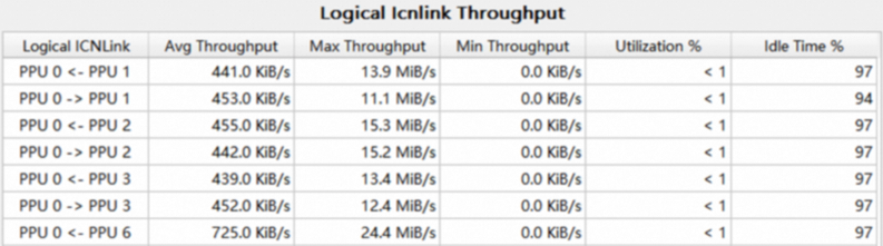
1.8 Launch statistics

This section lists the configuration for executing this kernel, including the grid size, block size, and PPU resource requirements.

The items in the header table are as follows:

The kernel's startup configuration directly affects occupancy. For optimal kernel performance, consider the following:

• A warp contains 32 threads, so the block size should be a multiple of 32.

• The grid size should be much larger than the number of CUs. If there are fewer blocks than CUs, some CUs will be idle. Consider reducing the block size or increasing the grid size.

• Use the waves per CU metric to check for a tail effect. If the waves per CU value is not an integer, the last wave cannot fully utilize the CU, reducing occupancy and degrading performance. Consider adjusting the block size to make the waves per CU value closer to an integer.

1.9 Occupancy

The Occupancy section shows kernel occupancy. Occupancy is the ratio of active warps to the maximum number of concurrent warps on a single CU. With enough warps, the PPU can switch between them to hide latency. High occupancy is essential for efficient kernel execution. The theoretical maximum number of active warps per CU is 64.

The number of active warps on a compute unit is limited by the following three factors:

• Block size

• Registers per thread

• Shared memory per block

1.9.1 Header table

The items in the table header are defined as follows:

1.9.2 Occupancy line chart

The occupancy section uses three line charts to illustrate how each of the three factors affects occupancy. In each chart, the x-axis represents the theoretical upper limit for one factor, while the y-axis shows the resulting theoretical occupancy. This calculation holds the other two factors constant at their actual values. The dot on the line indicates the current actual value. Hover over the dot to view its value.

1.10. Source counters

The source counters section helps you identify performance issues in your kernel code. This section contains three tables, each listing the lines of assembly code from the current kernel with the highest values for a specific metric: stall reasons, instructions executed, or thread instructions executed. Click a row to navigate to the source page. This helps you quickly pinpoint performance bottlenecks in your code.

• Warp Stall Sampling (All Samples)

• Warp Stall Sampling (Not Issued Samples)

• Most Instructions Executed

• Most Thread Instructions Executed

The first column lists the address and function name of each line of code. Click an entry to view details on the Source Page.

The second column shows the metric for the corresponding line of code. Hover over a cell to view a breakdown of the metric in the tooltip. For example, in the Warp Stall Sampling table, the tooltip shows the value and percentage for each stall reason.

The third column shows each row's metric value as a percentage of the total.

2. Source page

The Source Page displays the correlation between source code and assembly code. It also includes source-level metrics, such as stall reasons collected via Warp Sampling, instruction execution counts from instruction statistics, and live register metrics. Hover over the column headers for these metrics to view their detailed descriptions.

The Source Page supports syntax highlighting for assembly code, C++ code (including common GPU extension syntaxes), and Python code.

If an application is compiled with the -G or -lineinfo compiler option, the binary includes debug information. This information allows the tool to correlate source code with assembly when parsing the report.

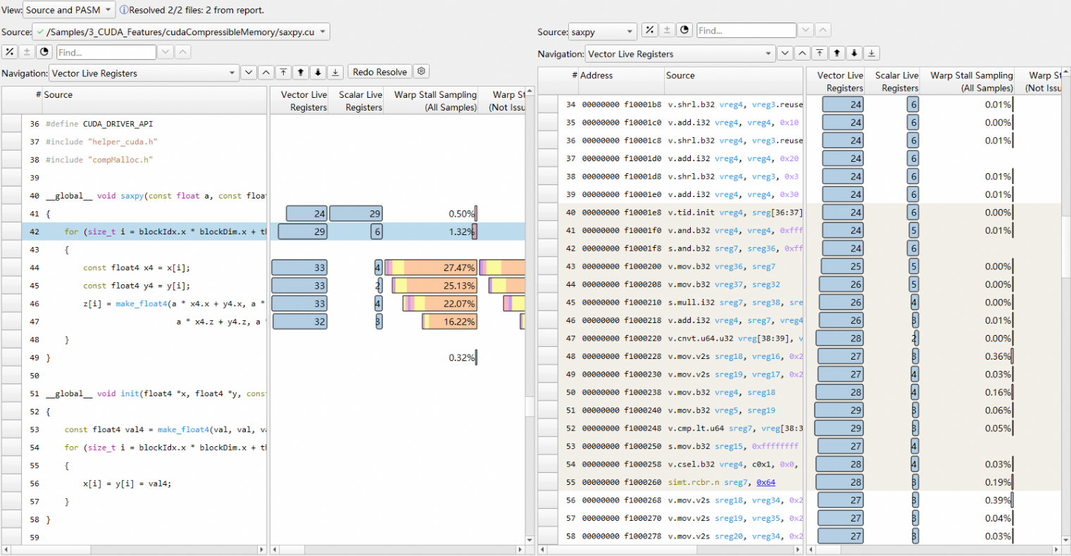
In the Source and PASM view, clicking a source code line highlights the corresponding assembly lines, and vice versa.

The Warp Stall Sampling (All Samples) metric aggregates all types of stall reasons. The Warp Stall Sampling (Not Issued Samples) metric aggregates stall reasons for instructions that were not issued. You can hover over a row in these columns to see a summary of the stall reasons for that line of code.

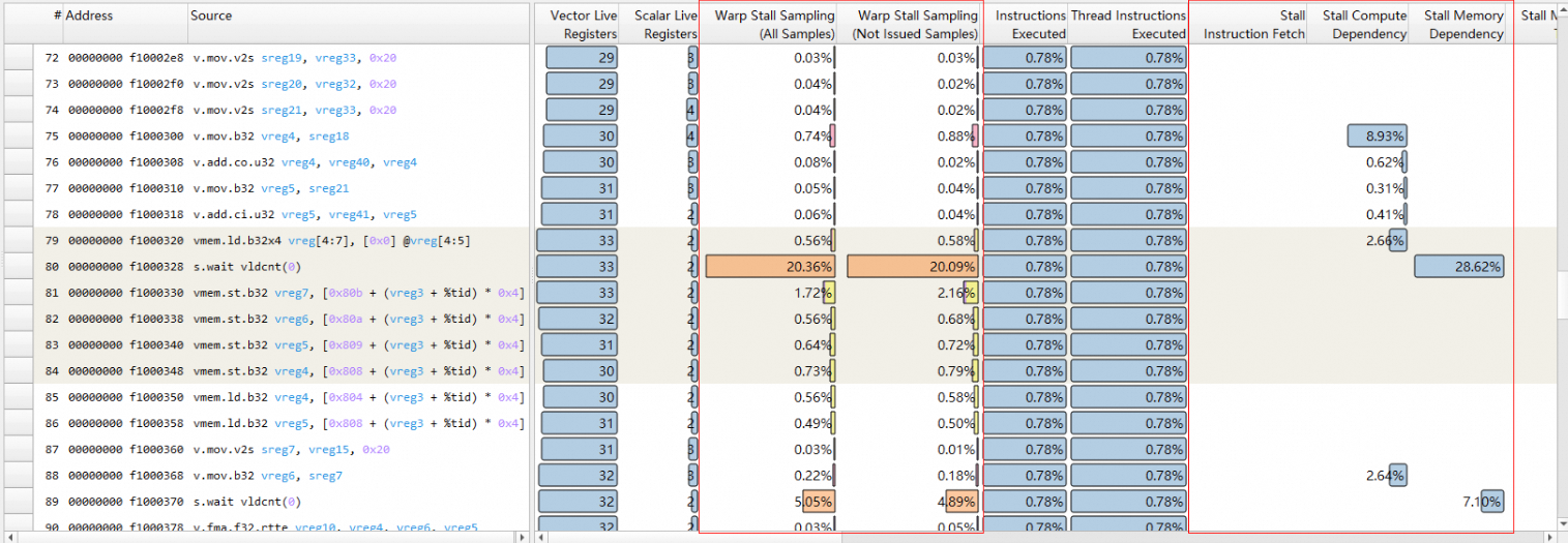
Hovering over the Warp Stall Sampling column displays detailed stall reason information:

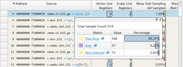
Instruction Executed and Thread Instruction Executed summarize the number of warps and threads that execute different instructions.

Vector Live Register and Scalar Live Register show the number of live vector or scalar registers used by each line of code.

2.1 Basic features

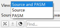
View dropdown menu

Use this dropdown menu to switch between the Source, PASM, and Source and PASM views.

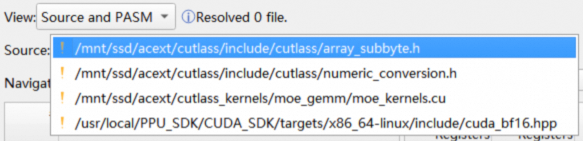
Source dropdown menu

Use this dropdown menu to switch between different source code files.

Source files are sorted by filename in ascending order; assembly functions are sorted by address in ascending order:

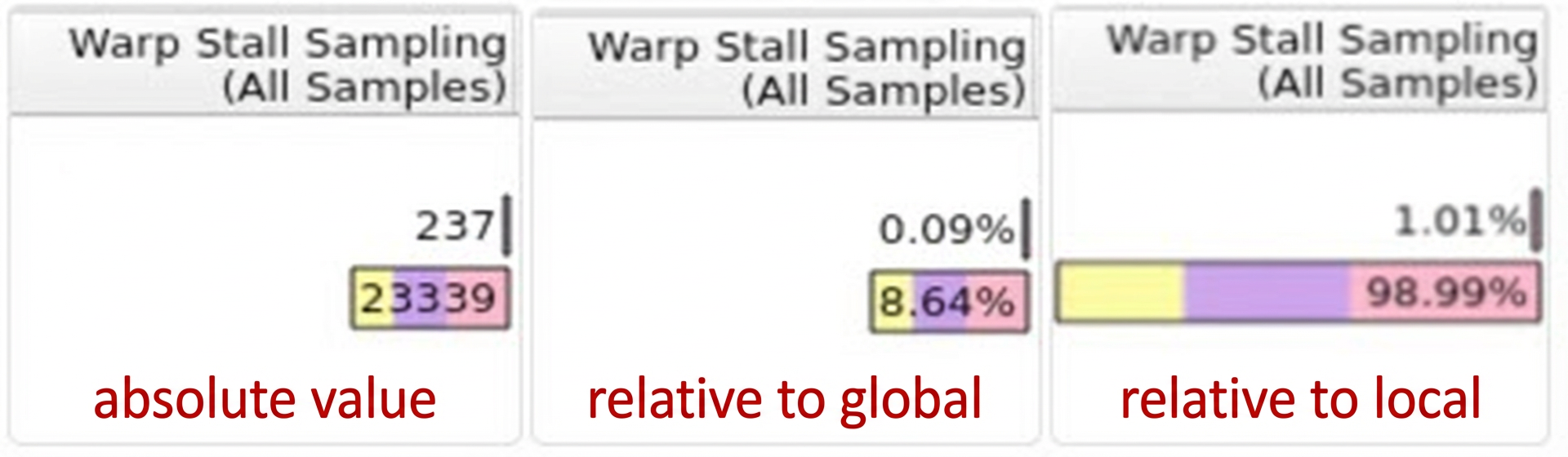
Metric display format buttons

Three buttons control the display style for metric columns. These settings apply to columns for instruction statistics and stall reasons:

1. Relative/Absolute value button

   • By default, Relative is selected, displaying metric values as a percentage of a total. The third button determines whether this total is local or global.

   

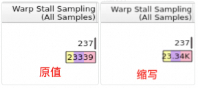
2. Abbreviated/Raw value button

   • This option is enabled only when Absolute is selected.

   • Abbreviated is selected by default. For example, the raw value 23339 is abbreviated as 23.34K.

   

3. Local/Global scope button

   • Local means percentages are relative to the sum of the metric's values for all code lines in the current source.

   • Global means percentages are relative to the sum of the metric's values for all code lines across all sources.

   • Global is selected by default.

Note: In the Source View, a source refers to a source code file. In the PASM View, a source refers to a function.

For example, consider a kernel with two source files: saxpy.cu and vector_functions.hpp. A line of code in saxpy.cu has an inst_executed metric value of 5. The total inst_executed value for all lines in saxpy.cu is 40, and the total for vector_functions.hpp is 60. In Local + Relative mode, the table shows 12.5% (5/40). In Global + Relative mode, the table shows 5% (5/100). In Absolute mode, the local/global setting is ignored, and the table displays the raw value, 5.

Each time you open a report, these options revert to their default settings. You can change the defaults for the first two options in the Options menu:

Changes to these defaults in Options do not apply to any Source Page that is already open.

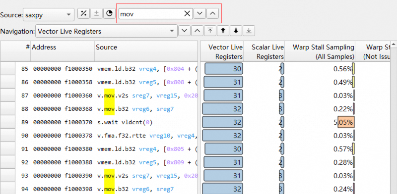
Find bar

Use the Find bar to quickly locate lines that contain a keyword. Enter a keyword to highlight all matches in yellow. Use the up and down buttons to jump to the previous or next match.

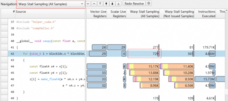
Navigation bar

Use the Navigation bar to jump between code lines that have a value for a specific metric. Use the up and down buttons to move to the previous or next matching line. For example, the following figure shows the result of using the down button to find and select the first line in saxpy.cu that has a Warp Stall Sampling (All Samples) value.

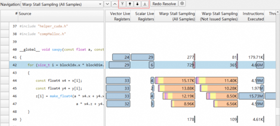
Metric sorting buttons

The metric sorting buttons let you quickly find the line with the maximum, next-largest, next-smallest, or minimum value for a given metric. For example, to find the line with the highest value for a metric, select the metric from the dropdown list and then click the Select Maximum button. To find the next-smallest value, click the Next Smallest button.

From left to right, the buttons are Select Maximum, Next Largest, Next Smallest, and Minimum.

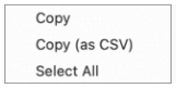
Context menu

The table in the Source Page supports the following options in the context menu:

• Copy: Copies the selected content to the clipboard.

• Copy as CSV: Copies the selected content to the clipboard in CSV format.

• Select All: Selects all content in the table.

Jump from branch instructions

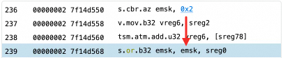
Click the address or offset in a branch instruction to jump to the target instruction's line. For example, for the instruction on line 236, s.cbr.az emsk, 0x2, clicking 0x2 skips the next two assembly instructions and jumps to line 239.

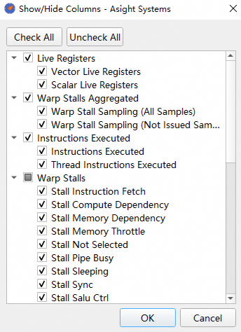
Show or hide specific columns

Open the column selector from the header's context menu to customize which columns to display:

2.2 Import source code

Include source code in the report

The acu tool can bundle source code into the report. To enable this, set the --import-source option to yes or on during collection. This option is disabled by default.

If a report includes source code, the Source Page automatically displays the corresponding code, and you do not need to import it manually.

Resolve

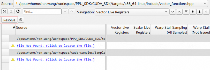
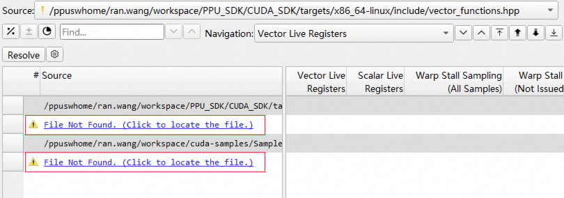
By default, a report does not include source code. When you open the Source Page, the tool attempts to import the source code from its original path at collection time. If this fails, a "File Not Found" message appears, and you must click Resolve to specify the source code directory. After you click Resolve, the tool first tries to import from the Source Lookup list. If that also fails, you can select a directory or file, and the tool then attempts to import other files using their relative paths.

Click the settings icon next to the Resolve button to open the Source Lookup window and configure preferred search paths.

You can also click the File Not Found link to open the resolve window.

The interface indicates where the source code was imported from, which can be one of three locations:

In the Source dropdown list, an icon next to each source file indicates whether it has been imported.

Redo Resolve

If a source file has already been imported, the Redo Resolve button in the Source View lets you re-select and re-import the current file.

Source Lookup

To specify fixed directories for importing source code, such as a permanent library path, use the Source Lookup feature. When you click Resolve, the tool prioritizes directories from the Source Lookup list. To manage source locations, navigate to Tools->Options...->Source Lookup or click the settings icon next to the Resolve button on the Source Page. In this menu, you can enable or disable added source locations with checkboxes and choose whether the Resolve button automatically saves new paths.

The menu button also lets you add, delete, and reorder the source code search paths.

3. Raw Page

The Raw Page displays all collected metrics for each kernel launch.

Sort

Click a metric column to sort it.

Filter

Enter a keyword in the Filter box to hide non-matching metric columns.

Transpose

The Raw Page supports table transposition, allowing you to view metrics as rows and kernels as columns.

Kernel comparison

Double-click a table cell to set the corresponding kernel as the current kernel.

After you add baselines, the values in the table update to the following difference format:

<focus value> (<difference to baselines average [%]>, z=<standard score>) (<number of values>)

Export

Use the menu in the top-right corner to export the Raw Page table to formats such as CSV.

Multi-instance metric format

Multi-instance metrics can be displayed in the table in two formats, which you can configure in the Options dialog:

• not instanced: totalValue {instanceCount}. For example, 12 {3}.

  • After adding a baseline, the format also shows the percentage difference, for example, 12 (+0.00%){3}.

  

• instanced: totalValue {value1; value2; ...}. For example, 12 (2; 4; 6).

  • After adding a baseline, the format also shows the percentage difference, for example, 12 (+0.00%)(2; 4; 6).

  

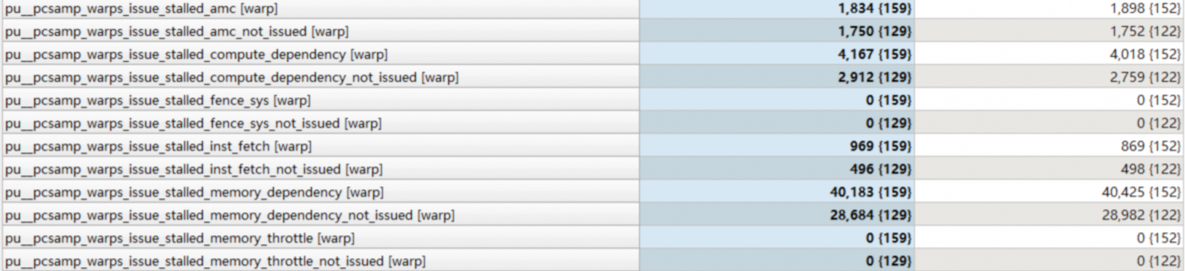
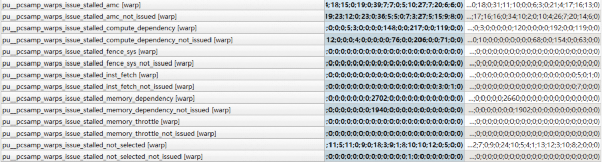
Multi-instance metrics belong to three main categories:

• number of instructions executed: inst_executed and thread_inst_executed.

• instruction category: sass__inst_executed_per_opcode.

• stall reason: pu__pcsamp_warps_issue_stalled*.

4. Summary page

The Summary Page displays key metrics for all collected kernel launches, offering a high-level overview to help you pinpoint kernels that require further analysis.

By default, this page displays ID, Time, API call ID, Function name, Demangled name, Process, Device name, Grid size, and Block size.

You can add metrics under Tools->Options->Profile->Report Summary Page. Use the format {customized_name:metric_name}, where metric_name is the metric's original name and customized_name is its display name. Separate multiple metrics with a comma.

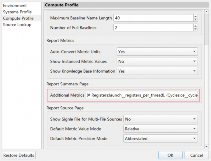
The features for sorting, filtering, transposing, comparing kernels, and exporting on the Summary Page are similar to those on the Raw Page. Additionally, double-clicking a row opens the Details Page, which shows detailed metrics.

5. Session page

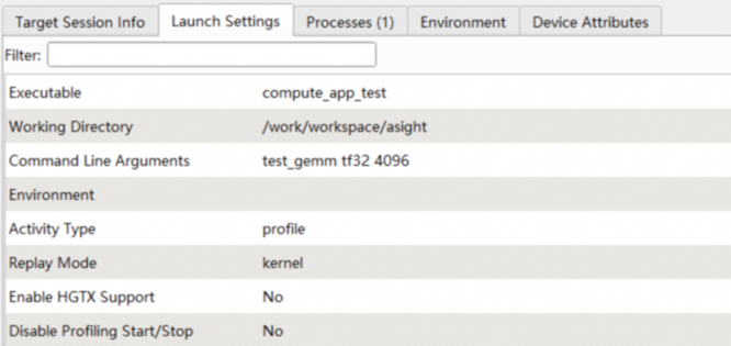
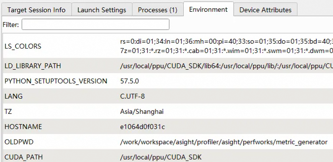
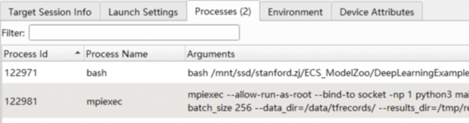
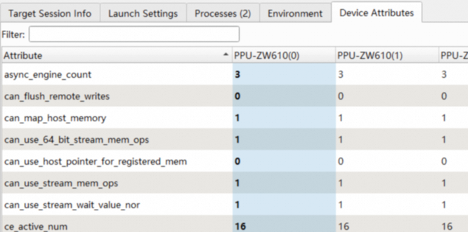
The Session Page presents a basic report in five sections: launch settings, session info, processes, environment, and device attributes. When you switch kernels, the Session Page highlights the device attributes for the selected kernel.

• Launch settings

  

• Session info

  

• Environment

  

• Processes

  

• Device attributes

  

6. Kernel filter

Asight Compute lets you filter kernel launches to narrow the results. Click Apply Filters to open the filter dialog box. You can use multiple filters to refine the list of kernel launches.

• Process: Filters kernel launches by their process ID. The default value is All.

• Launch name: Filters kernel launches by their launch name. This filter supports regular expressions with Perl-compatible syntax (disabled by default). If you do not select the "Regular expression" checkbox, the filter performs case-insensitive substring matching. If you select the checkbox, it performs a case-sensitive match based on the regular expression.

• Device ID: Filters kernel launches by their device ID. You can specify multiple device IDs, separated by a,.

The regular expression and device ID input fields include syntax validation. If your input is invalid, an error message appears and you cannot save the filter.

To clear all filters, click the dropdown arrow and select Clear Filters.

7. Baseline

Asight Compute provides a baseline feature to compare the profile results of multiple kernels, even across different reports.

1. The legend for the baselines. In a chart, each baseline is color-coded to match its legend entry.

2. The name of the baseline. You can rename a baseline by hovering over its name.

3. Adds the current kernel as a baseline.

4. Clears all baselines.

The appearance of baselines varies across different UI elements.

Baselines in charts

In addition to the current kernel, charts also display baselines. The color of each baseline corresponds to the legend.

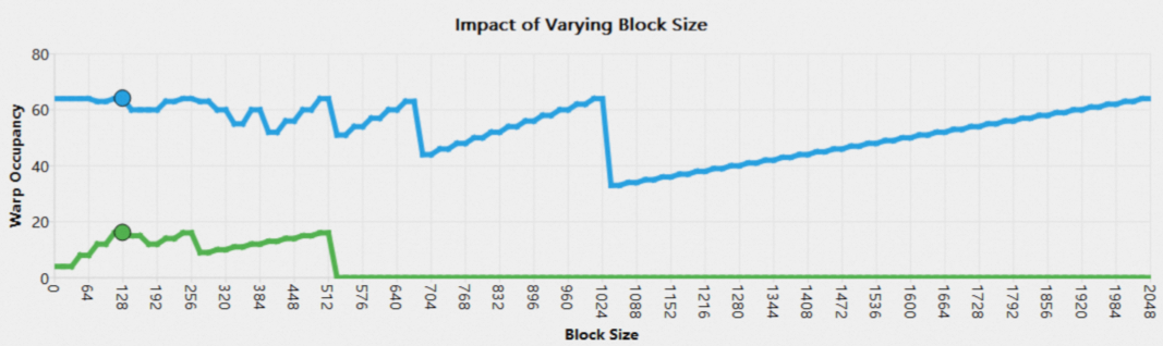
Tooltips in a chart also provide detailed baseline information.

Baselines in tables

When a single baseline is present, the table displays the percentage difference between the metrics of the current kernel and those of the baseline.

When more than one baseline is present, the table displays both the percentage difference in metrics and the standard score (z).

8. Occupancy calculator

The Occupancy Calculator Page lets you calculate the occupancy for a specific configuration and save the results to a file for later use. This page consists of two main parts: an input form and a results chart. The results chart is divided into three sections: Tables, Graphs, and GPU Data:

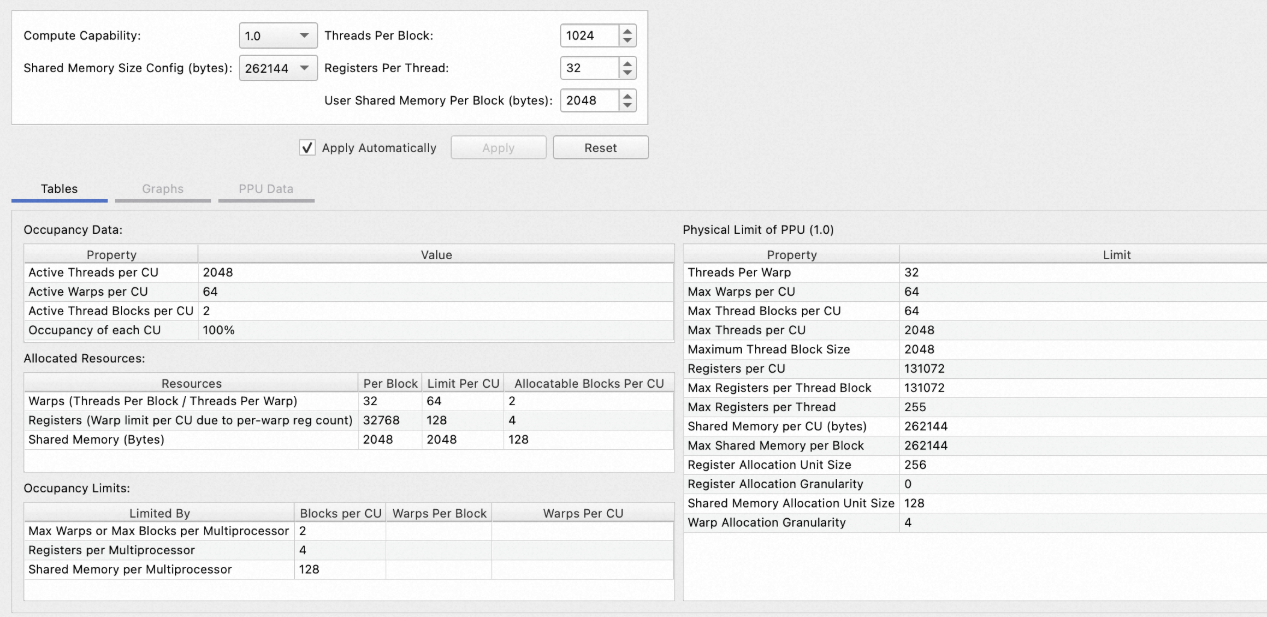
You can create or open a calculator in one of three ways:

• Click the Occupancy Calculator button at the top of the report.

  

• Click the calculator button next to the occupancy section.

  

• Open a saved .ncu-occ file by choosing File > Open.

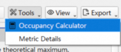
9. Metric details widget

To open the Metric Details widget on the right, select View->Metric Details from the main menu or click the Metric Details button at the top of the report:

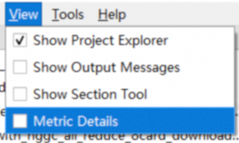
or

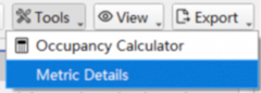
In an open report, click a metric on the Details page, Raw page, or Summary page to view its details in the Metric Details widget. The widget also lets you search for the details of a specific metric in the current report:

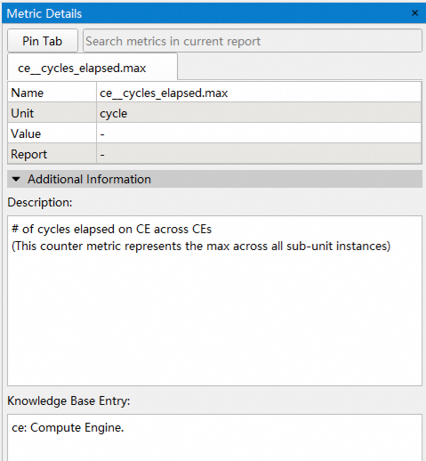
Metric details include the following sections:

• Metric information: The metric name, unit, value, and report.

• Additional information: The metric description and knowledgebase entry.

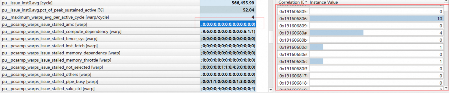
• Instance list: For metrics with multiple instances, the instance list lets you view the value for each instance. For example, open the Raw page and select the inst_executed metric to see the instruction execution count for each assembly code address. In addition to instruction execution count metrics (such as inst_executed and thread_inst_executed), instruction statistics metrics (sass__inst_executed_per_opcode) and stall reason metrics (pu__pcsamp_warps_issue_stalled*) are also multi-instance metrics.

After you click a metric in the report or search for one, the widget displays its details by default in the first tab (the Default tab). Click the Pin Tab button to pin the metric from the Default tab to a new, separate tab (a Pinned tab). This lets you temporarily store multiple metrics and switch between them for comparison.