
如果您的数据表经常需要进行GROUP BY、JOIN操作或为了避免数据倾斜,您可以在建表时设置分布键(Distribution Key),合适的分布键可以帮助数据均匀分布在所有计算节点上,显著提高计算和查询性能。本文为您介绍Hologres中为表设置Distribution Key。
Distribution Key介绍
在Hologres中,Distribution Key属性指定了表数据的分布策略,系统会保证Distribution Key相同的记录被分配到同一个Shard上。建表时设置语法如下:
-- Hologres V2.1版本起支持的语法
CREATE TABLE <table_name> (...) WITH (distribution_key = '[<columnName>[,...]]');
-- 所有版本支持的语法
BEGIN;
CREATE TABLE <table_name> (...);
call set_table_property('<table_name>', 'distribution_key', '[<columnName>[,...]]');
COMMIT;
参数说明如下:
|
参数 |
说明 |
|
table_name |
设置分布键的表名称。 |
|
columnName |
设置分布键的字段名称。 |
Distribution Key是非常重要的分布式概念,合理设置Distribution Key可以达到如下效果:
-
显著提高计算性能。
不同的Shard可以进行并行计算,从而提高计算性能。
-
显著提高每秒查询率(QPS)。
当您以Distribution Key做过滤条件时,Hologres可以直接筛选出数据相关的Shard进行扫描。否则Hologres需要让所有的Shard参与计算,影响QPS。
-
显著提高Join性能。
当两张表在同一个Table Group内,并且Join的字段是Distribution Key时,那么数据分布保证表A一个Shard内的数据和表B同一Shard内的数据对应,只需要直接在本节点Join本节点数据(Local Join)即可,可以显著提高执行效率。
使用建议
Distribution Key设置原则总结如下:
-
Distribution Key尽量选择分布均匀的字段,否则容易因为数据倾斜导致负载倾斜,使得查询效率变低,排查数据倾斜请参见查看Worker倾斜关系。
-
选择
Group By频繁的字段作为Distribution Key。 -
Join场景中,设置Join字段为Distribution Key,实现Local Join,避免数据Shuffle。同时进行Join的表需要在同一个Table Group内。
-
不建议为一个表设置多个Distribution Key,建议设置的Distribution Key不超过两个字段。设置多字段为Distribution Key,查询时若没有全部命中,容易出现数据Shuffle。避免使用两列值相同的字段作为分布键,否则会导致数据都分布在一个shard上,造成数据倾斜。
-
支持单列或者多列设置为Distribution Key,指定列时如设置单列,命令语句中不要保留多余空格;如设置多个列,则以半角逗号(,)分隔,同样不要保留多余空格。指定多列为Distribution Key时,列的顺序不影响数据的布局和查询性能。
-
表设置了主键(PK)时,Distribution Key必须为PK或者PK中的部分字段(不能为空,即不指定任何列),因为要求同一记录的数据只能属于一个Shard。如果没有额外指定Distribution Key,默认将PK设置为Distribution Key。
使用限制
-
设置Distribution Key需要在建表时设置,建表后如需修改Distribution Key需要重新建表并导入数据。
-
不支持修改Distribution Key对应列的值,如需修改请重新建表。
-
不支持将Float、Double、Numeric、Array、Json及其他复杂数据类型的字段设为Distribution Key。
-
表未设置PK时,Distribution Key没有限制,可以为空(不指定任何列)。如果为空,即随机Shuffle,数据随机分布到不同Shard上。从Hologres V1.3.28版本开始,Distribution Key禁止为空,示例用法如下。
--从1.3.28版本开始,写法将会被禁止 CALL SET_TABLE_PROPERTY('<tablename>', 'distribution_key', ''); -
Distribution Key列的值中有
null时,当作“”(空串)看待,即Distribution Key为空。
技术原理
Distribution Key指定了表的分布策略。根据实际的业务场景,存在以下情形。
设置Distribution Key
为表设置了Distribution Key之后,数据会根据Distribution Key被分配到各个Shard上,算法为Hash(distribution_key)%shard_count,结果为对应的Shard。系统会保证Distribution Key相同的记录会被分配到同一个Shard上,示例如下。
-
V2.1版本起支持的建表语法:
--设置a列为distribution key,系统会对a列的值做hash操作,再取模,即hash(a)%shard_count = shard_id,结果相同的一组数据分布在同一个Shard内 CREATE TABLE tbl ( a int NOT NULL, b text NOT NULL ) WITH ( distribution_key = 'a' ); --设置a、b两列为distribution key,系统对a,b两个列的值做hash操作,再取模,即hash(a,b)%shard_count = shard_id,结果相同的一组数据分布在同一个Shard内 CREATE TABLE tbl ( a int NOT NULL, b text NOT NULL ) WITH ( distribution_key = 'a,b' ); -
所有版本支持的建表语法:
--设置a列为distribution key,系统会对a列的值做hash操作,再取模,即hash(a)%shard_count = shard_id,结果相同的一组数据分布在同一个Shard内
begin;
create table tbl (
a int not null,
b text not null
);
call set_table_property('tbl', 'distribution_key', 'a');
commit;
--设置a、b两列为distribution key,系统对a,b两个列的值做hash操作,再取模,即hash(a,b)%shard_count = shard_id,结果相同的一组数据分布在同一个Shard内
begin;
create table tbl (
  a int not null,
  b text not null
);
call set_table_property('tbl', 'distribution_key', 'a,b');
commit;
数据分布示意图如下: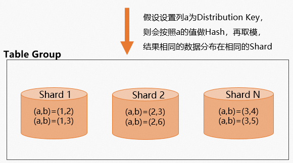 但在设置Distribution Key时,需要关注设置为Distribution Key字段的数据最好是分布均匀的。Hologres的Shard数和Worker节点数有一定的关联关系,详情请参见基本概念。如果设置了数据分布不均匀的字段作为Distribution Key之后,那么数据会集中分布在某些Shard上,导致大部分的计算集中到部分Worker上,出现长尾效应,查询效率降低。排查以及处理数据的倾斜情况详情请参见查看Worker倾斜关系。
不设置Distribution Key
不设置Distribution Key时,数据将会被随机分布在各个Shard,相同的数据可能会在相同Shard,也可能在不同的Shard,示例如下。
--不设置distribution key
begin;
create table tbl (
a int not null,
b text not null
);
commit;
数据分布示意图如下: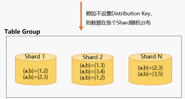
Group By聚合场景设置Distribution Key
为表设置了Distribution Key,那么相同的数据就分布在相同的Shard上,同时对于Group By聚合场景,数据在计算时按照设置的Distribution Key重新分布,因此可以将Group By频繁的字段设置为Distribution Key,这样数据在Shard内就已经聚合,减少数据在Shard间的重分配,提高查询性能,示例如下。
-
V2.1版本起支持的建表语法:
CREATE TABLE agg_tbl ( a int NOT NULL, b int NOT NULL ) WITH ( distribution_key = 'a' ); --示例查询,对a列做聚合查询 select a,sum(b) from agg_tbl group by a; -
所有版本支持的建表语法:
begin;
create table agg_tbl (
a int not null,
b int not null
);
call set_table_property('agg_tbl', 'distribution_key', 'a');
commit;
--示例查询,对a列做聚合查询
select a,sum(b) from agg_tbl group by a;
通过查看执行计划(explain SQL),执行计划结果中没有redistribution算子,说明数据没有重分布。执行该查询的执行计划结果为:顶层算子 Gather(cost=0.00..5.53, rows=10000, width=12),下层 HashAggregate(cost=0.00..5.24, rows=10000, width=12,Group Key: a),再下层依次为 Exchange (Gather Exchange)、Decode、Seq Scan on agg_tbl。优化器为 HQO version 1.3.0。该计划表明数据按 Distribution Key a 分布后,HashAggregate 直接在 Shard 内按 a 完成聚合,无需跨 Shard 重分布。
两表关联场景设置Distribution Key
-
两表Join字段设置为Distribution Key
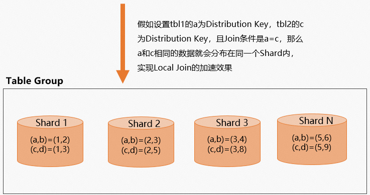
在两表关联(Join)的场景,如果两表Join字段分别在对应表里都设置为Distribution Key,那么Join字段相同的数据就会分布在相同的Shard,这样就能实现Local Join,从而实现查询加速的效果,示例如下。
-
建表DDL。
-
V2.1版本起支持的建表语法:
--tbl1按照a列分布,tbl2按照c列分布,当tbl1与tbl2以a=c关联条件join时,对应的数据分布在同一个Shard内,这种查询可以实现Local Join的加速效果 BEGIN; CREATE TABLE tbl1 ( a int NOT NULL, b text NOT NULL ) WITH ( distribution_key = 'a' ); CREATE TABLE tbl2 ( c int NOT NULL, d text NOT NULL ) WITH ( distribution_key = 'c' ); COMMIT; -
所有版本支持的建表语法:
--tbl1按照a列分布,tbl2按照c列分布,当tbl1与tbl2以a=c关联条件join时,对应的数据分布在同一个Shard内,这种查询可以实现Local Join的加速效果
begin;
create table tbl1(
a int not null,
b text not null
);
call set_table_property('tbl1', 'distribution_key', 'a');
create table tbl2(
c int not null,
d text not null
);
call set_table_property('tbl2', 'distribution_key', 'c');
commit;
-
-
查询语句。
select * from tbl1 join tbl2 on tbl1.a=tbl2.c;
数据分布示意图如下。
 通过查看执行计划(explain SQL),如下所示执行计划结果中没有
redistribution算子,说明数据没有重分布。QUERY PLAN Gather (cost=0.00..10.27 rows=1000 width=24) -> Hash Join (cost=0.00..10.21 rows=1000 width=24) Hash Cond: (tbl1.a = tbl2.c) -> Exchange (Gather Exchange) (cost=0.00..5.10 rows=1000 width=12) -> Decode (cost=0.00..5.10 rows=1000 width=12) -> Seq Scan on tbl1 (cost=0.00..5.00 rows=1000 width=12) -> Hash (cost=5.10..5.10 rows=1000 width=12) -> Exchange (Gather Exchange) (cost=0.00..5.10 rows=1000 width=12) -> Decode (cost=0.00..5.10 rows=1000 width=12) -> Seq Scan on tbl2 (cost=0.00..5.00 rows=1000 width=12) Optimizer: HQO version 1.3.0 -
-
两表Join字段未都设置为Distribution Key
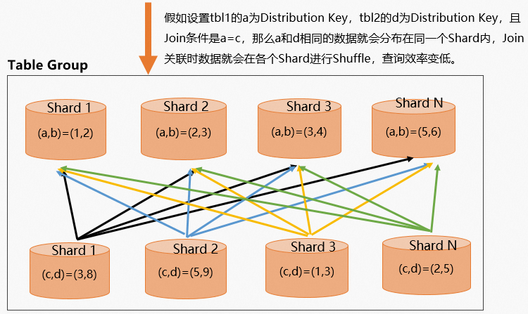
在两表关联(Join)的场景,如果两表Join字段在对应表里未都设置为Distribution Key,那么查询时数据就会在各个Shard Shuffle(执行计划会根据关联的两个表大小,来判断是进行Shuffle还是Broadcast)。如下示例,设置
tbl1的a字段为Distribution Key,tbl2的d字段为Distribution Key,而Join条件是a=c,那么c字段就会在每个Shard Shuffle一遍,从而导致查询效率变低。-
建表DDL。
-
V2.1版本起支持的建表语法:
BEGIN; CREATE TABLE tbl1 ( a int NOT NULL, b text NOT NULL ) WITH ( distribution_key = 'a' ); CREATE TABLE tbl2 ( c int NOT NULL, d text NOT NULL ) WITH ( distribution_key = 'd' ); COMMIT; -
所有版本支持的建表语法:
begin;
create table tbl1(
a int not null,
b text not null
);
call set_table_property('tbl1', 'distribution_key', 'a');
create table tbl2(
c int not null,
d text not null
);
call set_table_property('tbl2', 'distribution_key', 'd');
commit;
-
-
查询语句。
select * from tbl1 join tbl2 on tbl1.a=tbl2.c;
数据分布示意图如下。
 通过查看执行计划(explain SQL),如下所示执行计划中有
redistribution算子,说明数据进行了重分布,表明Distribution Key设置的不合理,需要重新设置。执行以上查询语句的执行计划如下,可以看到存在Redistribution(数据重分布)操作,说明Distribution Key不一致导致了额外的数据搬移:QUERY PLAN Gather (cost=0.00..10.27 rows=1000 width=24) -> Hash Join (cost=0.00..10.21 rows=1000 width=24) Hash Cond: (tbl2.c = tbl1.a) -> Redistribution (cost=0.00..5.10 rows=1000 width=12) Hash Key: tbl2.c -> Exchange (Gather Exchange) (cost=0.00..5.10 rows=1000 width=12) -> Decode (cost=0.00..5.10 rows=1000 width=12) -> Seq Scan on tbl2 (cost=0.00..5.00 rows=1000 width=12) -> Hash (cost=5.10..5.10 rows=1 width=12) -> Exchange (Gather Exchange) (cost=0.00..5.10 rows=1 width=12) -> Decode (cost=0.00..5.10 rows=1 width=12) -> Seq Scan on tbl1 (cost=0.00..5.00 rows=1 width=12) Optimizer: HQO version 1.3.0 -
多表关联场景设置Distribution Key
多表关联的场景比较复杂,可以遵循如下原则:
-
每个表的Join字段都相同,那么将Join字段都设置为Distribution Key。
-
每个表的Join字段不同,优先考虑大表间的Join,将大表的Join字段设置为Distribution Key。
通过以下几种情况举例说明(本文中以三个表Join为例说明,大于三个表的Join情况可以参考本示例)。
-
三个表的Join字段相同
在三个表Join的场景中,三个表的Join字段都相同,那么这种情况是最简单的,可以直接将三个表的Join字段都设置为Distribution Key,实现Local Join的能力。
-
V2.1版本起支持的建表语法:
BEGIN; CREATE TABLE join_tbl1 ( a int NOT NULL, b text NOT NULL ) WITH ( distribution_key = 'a' ); CREATE TABLE join_tbl2 ( a int NOT NULL, d text NOT NULL, e text NOT NULL ) WITH ( distribution_key = 'a' ); CREATE TABLE join_tbl3 ( a int NOT NULL, e text NOT NULL, f text NOT NULL, g text NOT NULL ) WITH ( distribution_key = 'a' ); COMMIT; --3表join查询 SELECT * FROM join_tbl1 INNER JOIN join_tbl2 ON join_tbl2.a = join_tbl1.a INNER JOIN join_tbl3 ON join_tbl2.a = join_tbl3.a; -
所有版本支持的建表语法:
begin;
create table join_tbl1(
a int not null,
b text not null
);
call set_table_property('join_tbl1', 'distribution_key', 'a');
create table join_tbl2(
a int not null,
d text not null,
e text not null
);
call set_table_property('join_tbl2', 'distribution_key', 'a');
create table join_tbl3(
a int not null,
e text not null,
f text not null,
g text not null
);
call set_table_property('join_tbl3', 'distribution_key', 'a');
commit;
--3表join查询
SELECT * FROM join_tbl1
INNER JOIN join_tbl2 ON join_tbl2.a = join_tbl1.a
INNER JOIN join_tbl3 ON join_tbl2.a = join_tbl3.a;
通过查看执行计划(explain SQL),如下所示执行计划中:
-
没有
redistribution算子,说明数据没有重分布,实现了Local Join。 -
exchange算子代表文件级别聚合到Shard级别聚合,这样就只需要对应Shard的数据,提升数据的查询效率。
QUERY PLAN Gather (cost=0.00..16.44 rows=10000 width=36) -> Hash Join (cost=0.00..15.57 rows=10000 width=36) Hash Cond: ((join_tbl2.a = join_tbl3.a) AND (join_tbl1.a = join_tbl3.a)) -> Hash Join (cost=0.00..10.31 rows=10000 width=20) Hash Cond: (join_tbl2.a = join_tbl1.a) -> Exchange (Gather Exchange) (cost=0.00..5.11 rows=10000 width=12) -> Decode (cost=0.00..5.11 rows=10000 width=12) -> Seq Scan on join_tbl2 (cost=0.00..5.00 rows=10000 width=12) -> Hash (cost=5.11..5.11 rows=10000 width=8) -> Exchange (Gather Exchange) (cost=0.00..5.11 rows=10000 width=8) -> Decode (cost=0.00..5.11 rows=10000 width=8) -> Seq Scan on join_tbl1 (cost=0.00..5.00 rows=10000 width=8) -> Hash (cost=5.12..5.12 rows=10000 width=16) -> Exchange (Gather Exchange) (cost=0.00..5.12 rows=10000 width=16) -> Decode (cost=0.00..5.12 rows=10000 width=16) -> Seq Scan on join_tbl3 (cost=0.00..5.00 rows=10000 width=16) Optimizer: HQO version 1.3.0 -
-
三个表的Join字段不同
在实际业务中,多表关联时会有Join字段不相同的场景,这个时候可以根据如下原则来设置Distribution Key:
-
核心优化原则是优先考虑大表间的Join,设置大表的Join字段为Distribution Key;小表因其数据量较少,无需过多考虑。
-
表数据量大致相同的情况,可以设置Group By频繁的Join字段为Distribution Key。
如下示例,有三个表相互Join,Join的字段不完全一样,这个时候选择大表的Join字段为Distribution Key,
join_tbl_1这个表数据量有一千万条,join_tbl_2和join_tbl_3分别有一百万条,以join_tbl_1为主要优化对象。-
V2.1版本起支持的建表语法:
BEGIN; -- join_tbl_1为1kw数据量 CREATE TABLE join_tbl_1 ( a int NOT NULL, b text NOT NULL ) WITH ( distribution_key = 'a' ); -- join_tbl_2为100w数据量 CREATE TABLE join_tbl_2 ( a int NOT NULL, d text NOT NULL, e text NOT NULL ) WITH ( distribution_key = 'a' ); -- join_tbl_3为100w数据量 CREATE TABLE join_tbl_3 ( a int NOT NULL, e text NOT NULL, f text NOT NULL, g text NOT NULL ); WITH ( distribution_key = 'a' ); COMMIT; --join key不相同时,选择大表的join key为distribution key。 SELECT * FROM join_tbl_1 INNER JOIN join_tbl_2 ON join_tbl_2.a = join_tbl_1.a INNER JOIN join_tbl_3 ON join_tbl_2.d = join_tbl_3.f; -
所有版本支持的建表语法:
begin;
--join_tbl_1为1kw数据量
create table join_tbl_1(
a int not null,
b text not null
);
call set_table_property('join_tbl_1', 'distribution_key', 'a');
--join_tbl_2为100w数据量
create table join_tbl_2(
a int not null,
d text not null,
e text not null
);
call set_table_property('join_tbl_2', 'distribution_key', 'a');
--join_tbl_3为100w数据量
create table join_tbl_3(
a int not null,
e text not null,
f text not null,
g text not null
);
--call set_table_property('join_tbl_3', 'distribution_key', 'a');
commit;
--join key不相同时,选择大表的join key为distribution key。
SELECT * FROM join_tbl_1
INNER JOIN join_tbl_2 ON join_tbl_2.a = join_tbl_1.a
INNER JOIN join_tbl_3 ON join_tbl_2.d = join_tbl_3.f;
通过查看执行计划(explain SQL),如下所示执行计划表明:
-
在
join_tbl_2和join_tbl_3表之间有redistribution算子,因为join_tbl_3是小表,Join字段与Distribution Key不一致,所以数据进行了重分布。 -
join_tbl_1和join_tbl_2表之间没有redistribution算子,因为两表将Join字段都设置为Distribution Key,因此数据不会重分布。
QUERY PLAN Gather (cost=0.00..183.90 rows=1000000 width=49) -> Hash Join (cost=0.00..64.87 rows=1000000 width=49) Hash Cond: (join_tbl_2.d = join_tbl_3.f) -> Redistribution (cost=0.00..40.22 rows=1000000 width=27) Hash Key: join_tbl_2.d -> Hash Join (cost=0.00..35.99 rows=1000000 width=27) Hash Cond: (join_tbl_1.a = join_tbl_2.a) -> Exchange (Gather Exchange) (cost=0.00..18.45 rows=10000000 width=11) -> Decode (cost=0.00..18.08 rows=10000000 width=11) -> Seq Scan on join_tbl_1 (cost=0.00..7.75 rows=10000000 width=11) -> Hash (cost=6.93..6.93 rows=1000000 width=16) -> Exchange (Gather Exchange) (cost=0.00..6.93 rows=1000000 width=16) -> Decode (cost=0.00..6.88 rows=1000000 width=16) -> Seq Scan on join_tbl_2 (cost=0.00..5.29 rows=1000000 width=16) -> Hash (cost=10.97..10.97 rows=1000000 width=22) -> Redistribution (cost=0.00..10.97 rows=1000000 width=22) Hash Key: join_tbl_3.f -> Exchange (Gather Exchange) (cost=0.00..7.53 rows=1000000 width=22) -> Decode (cost=0.00..7.45 rows=1000000 width=22) -> Seq Scan on join_tbl_3 (cost=0.00..5.31 rows=1000000 width=22) Optimizer: HQO version 1.3.0 -
使用示例
-
V2.1版本起支持的建表语法:
--单表设置为distribution key CREATE TABLE tbl ( a int NOT NULL, b text NOT NULL ) WITH ( distribution_key = 'a' ); --设置多个distribution key CREATE TABLE tbl ( a int NOT NULL, b text NOT NULL ) WITH ( distribution_key = 'a,b' ); --join场景,设置join key为distribution key BEGIN; CREATE TABLE tbl1 ( a int NOT NULL, b text NOT NULL ) WITH ( distribution_key = 'a' ); CREATE TABLE tbl2 ( c int NOT NULL, d text NOT NULL ) WITH ( distribution_key = 'c' ); COMMIT; SELECT b, count(*) FROM tbl1 JOIN tbl2 ON tbl1.a = tbl2.c GROUP BY b; -
所有版本支持的建表语法:
--设置一个distribution key
begin;
create table tbl (a int not null, b text not null);
call set_table_property('tbl', 'distribution_key', 'a');
commit;
--设置多个distribution key
begin;
create table tbl (a int not null, b text not null);
call set_table_property('tbl', 'distribution_key', 'a,b');
commit;
--join场景,设置join key为distribution key
begin;
create table tbl1(a int not null, b text not null);
call set_table_property('tbl1', 'distribution_key', 'a');
create table tbl2(c int not null, d text not null);
call set_table_property('tbl2', 'distribution_key', 'c');
commit;
select b, count(*) from tbl1 join tbl2 on tbl1.a = tbl2.c group by b;