Configure a workbook
This topic describes how to configure a workbook on the workbook editing page.
Prerequisites
You have logged on to the Quick BI console and created a workbook. For more information, see Create a workbook.
Top menu bar
You can perform the following operations in the top menu bar:

① Customize the workbook name.
② Add the workbook to your favorites.
③ Switch between PC and mobile view.
④ Lock or unlock the workbook.
⑤ Replace the dataset.
⑥ Configure global parameters for the workbook.
⑦ Page settings.

Display watermarks: Select this option to show watermarks.
Display analysis mode switch: Enables analysis mode in Preview.
When selected, formulas are recalculated after all data from query controls is retrieved.
Allow download: Allows users to export the workbook and configures how hidden rows and columns are handled during export. You can choose one of the following three options:
Export hidden rows, columns, and formulas: Exports hidden rows and columns, including their calculation formulas.
Export hidden rows and columns, values only: Exports hidden rows and columns, but converts formulas to their resulting values.
Do not export hidden rows and columns: Does not export hidden rows and columns.
Deferred formula calculation: If selected, formula calculation waits until all dependent datasets have finished loading. You can apply this setting to the initial sheet or the entire workbook.
Remember query conditions: If selected, the system remembers the query conditions.
Display row and column headers: If selected, row numbers and column letters are visible in Preview mode.

Dark mode: When enabled, a dark theme is applied to the workbook area and charts.
Allow submission only through data entry tasks: When enabled, users can only submit data through data entry tasks. They cannot submit data if they open the workbook directly from the workspace.
Global parameters: Configure global parameters for the workbook.
⑧ Switch between Preview and Edit modes.
Click Preview to enter Preview mode, which supports both PC and mobile layouts.
If you have configured group settings, you can view them in Preview mode and show or hide them as needed.
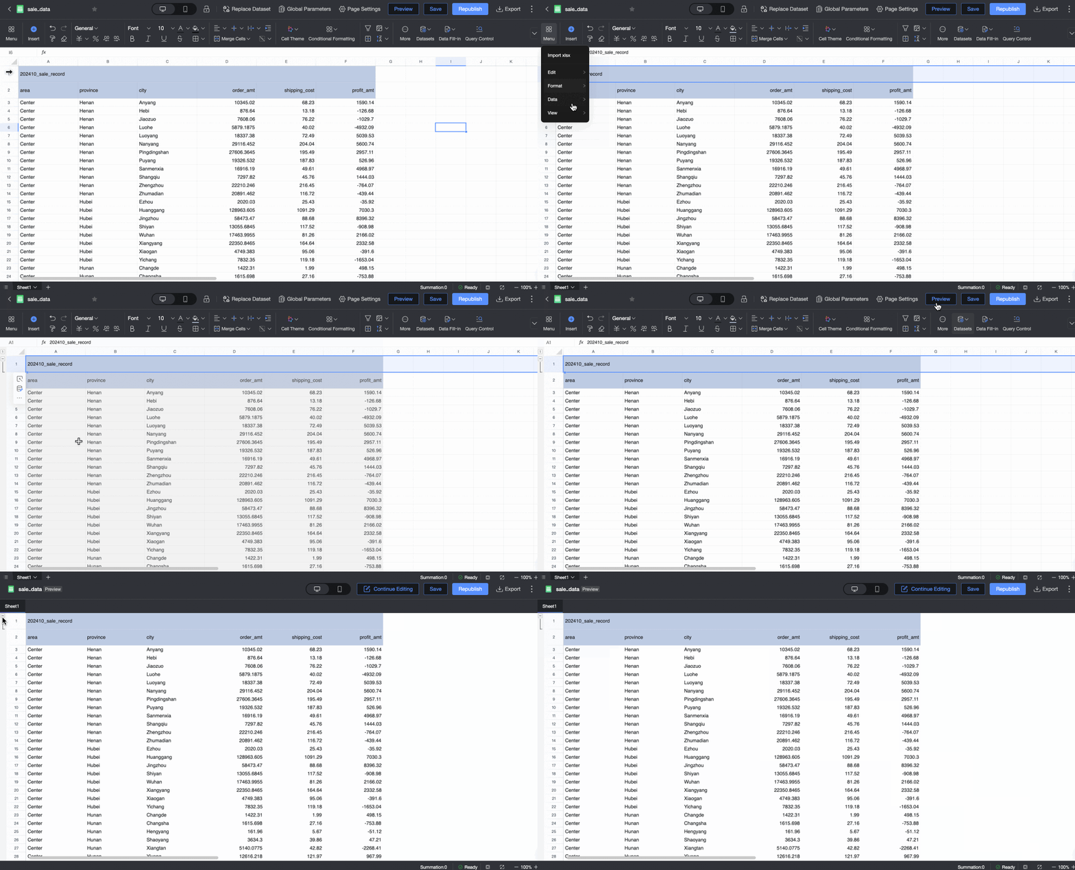
⑨ Save
⑩ Save and publish or republish the workbook.
⑪ Export the workbook: Export the current workbook as an Excel or PDF file to your local computer for offline viewing. Click the
 icon to configure the following settings in the Export dialog box.
Parameter
Description
Export name
The name of the exported workbook file. This name is automatically generated and cannot be modified. The naming convention is determined by the settings in Export Control. For more information, see Export Control.
File format
Set the format of the exported file. You can select EXCEL or PDF.
EXCEL: Only data from chart components can be exported in Excel format. For best compatibility, we recommend opening the exported file with Microsoft Excel.
PDF: Embedded pages and images that do not allow cross-origin access cannot be exported. Text gradients are not supported and are rendered as solid colors.
Export scope
Select the range of sheets to export from the current workbook.
All sheets: Export all sheets in the current workbook.
Current sheet: Export only the currently active sheet.
Custom range: Select specific sheets to export from the drop-down list.
Content scope
Select the content range to export from the workbook.
General: Export the raw data from the workbook without any filter information.
With Filter Condition Markers: Export with a screenshot of the query control information from the current sheet, such as date filters and product type filters.
Export channel
Specifies the destination for the exported file. The available channels are determined by the settings in Export Control. For more information, see Export Control.
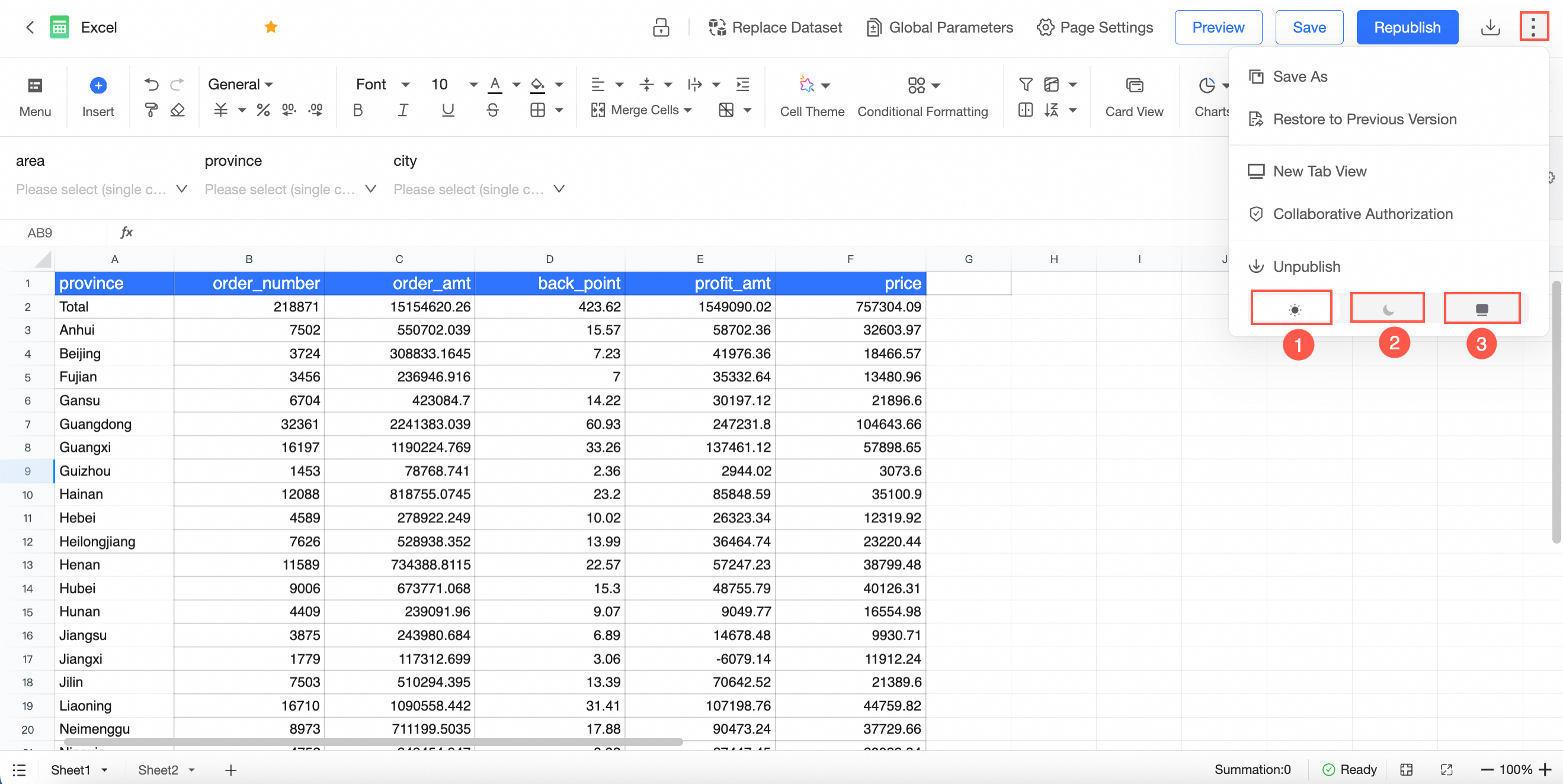
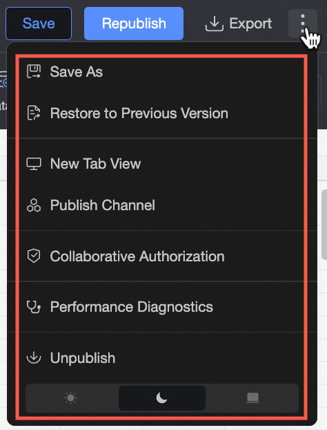
⑫ Save As, Restore Historical Version, Open in New Tab, Grant Permissions, Take Offline, and switch between light and dark modes.


Menu
In the menu, you can perform the following operations on the workbook:
② Edit
③ Format
④ Data
⑤ View
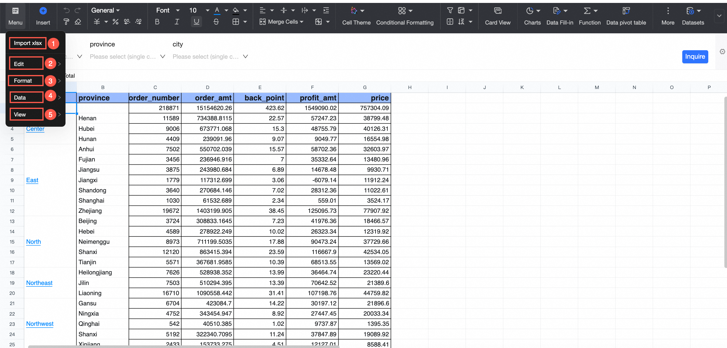
Import an .xlsx file
Imports an .xlsx file, overwriting the data in the current sheet.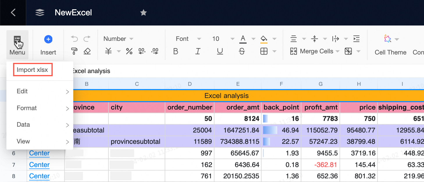
Edit
You can perform the following editing operations on the data in your workbook: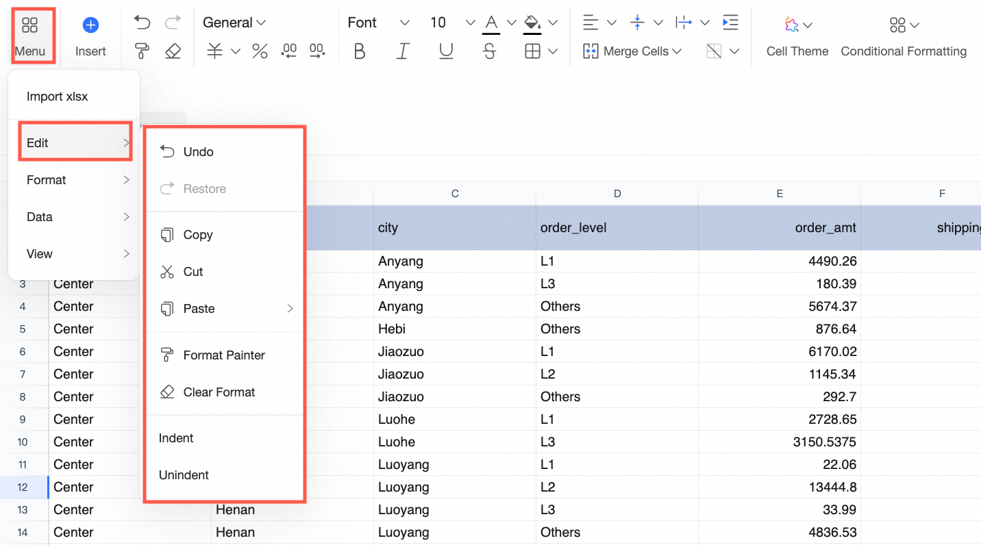
Insert
You can insert the following items into your workbook:
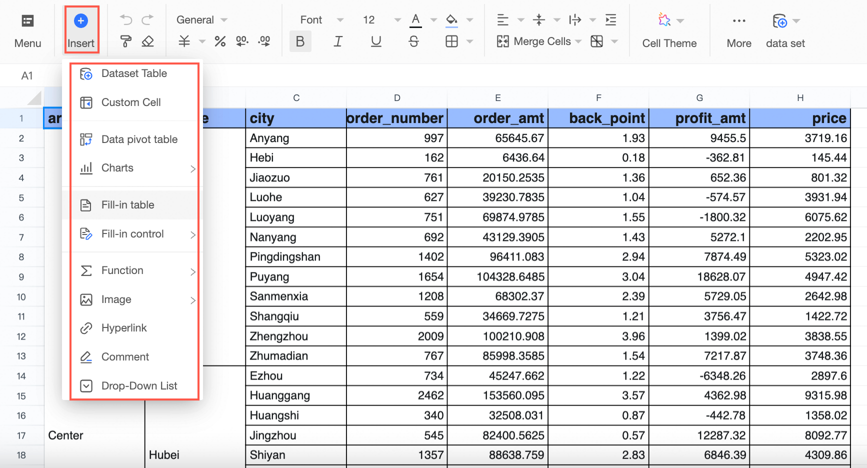
Dataset table
For more information, see Insert a dataset table.
Freestyle cell
For more information, see Insert a freestyle cell.
Pivot table: Insert a pivot table into the workbook.
For more information, see Insert a pivot table.
Charts: Insert a chart into the workbook.
Currently, line, column, pie, gauge, radar, scatter, funnel, and rose charts are supported. For more information, see Insert a chart.
Data entry table
For more information, see Table-based data entry.
Data entry controls
For more information, see Data entry controls.
Function: Insert a function into the workbook.
For more information, see Workbook functions.
Image: You can insert a floating image or an image in a cell.
NoteYou can use a shortcut key such as Ctrl+V (Windows) or Command+V (macOS) to paste an image into a cell.
The size of an inserted image cannot exceed 3 MB.
Currently, PNG, JPG, and GIF formats are supported.
Hyperlink: Add a hyperlink to the workbook.
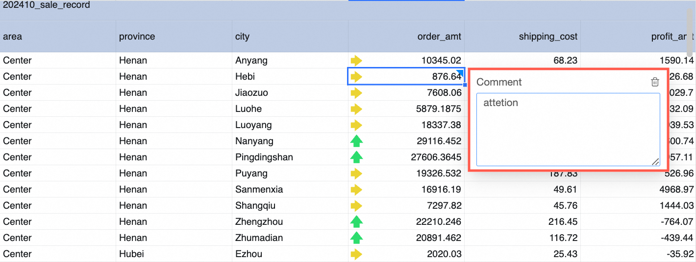
Comment: Add a comment to the workbook.
Drop-down list: Set custom values for a cell in the workbook.
For more information, see Add a drop-down list.
Format
You can set the format of content in the workbook.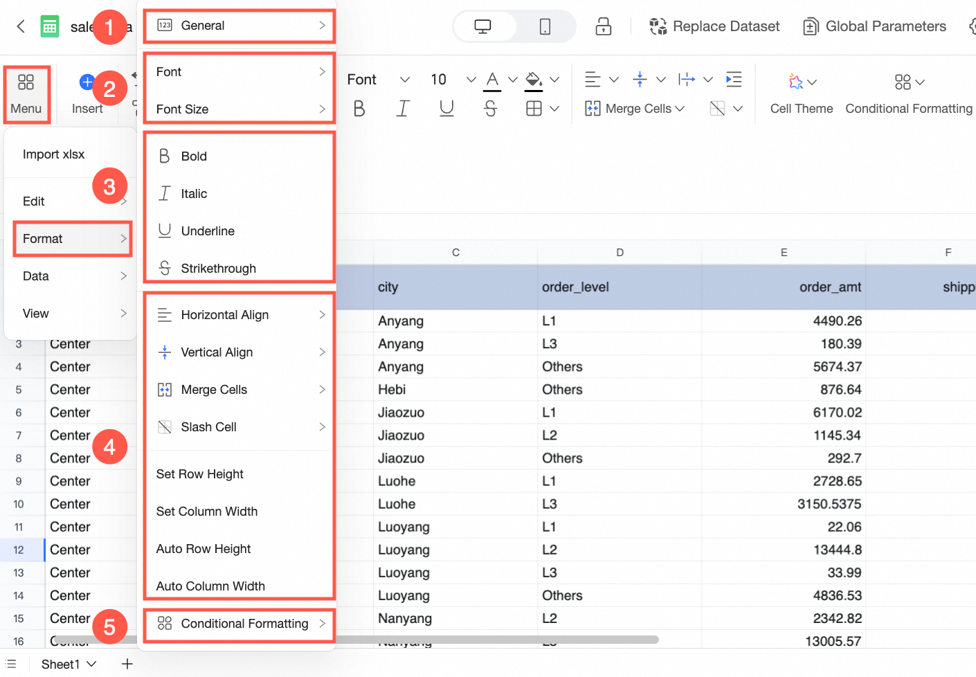
① Set the data format. Options include General, Text, Number, Currency, Date, Time, DateTime, Percent, and Custom. | ② Specify the font and font size. | ③ Specify the text style. |
④ Specify the cell style. | ⑤ Add rules for data results. For more information, see conditional formatting. | - |
Data
You can sort, filter, and search for data in the workbook.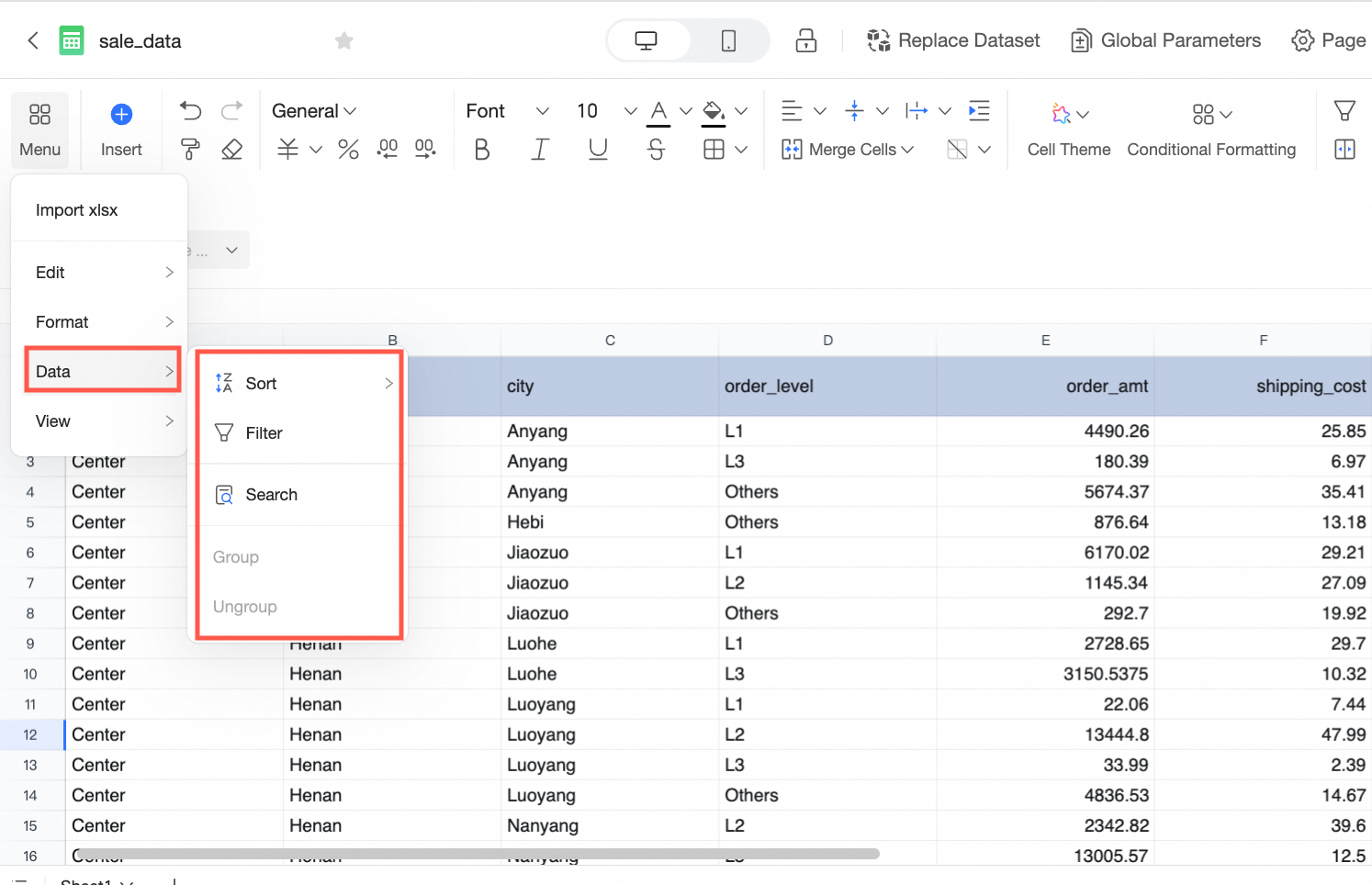
Option | Description |
Sort | Supports ascending, descending, and custom sorting. For more information, see Sort. |
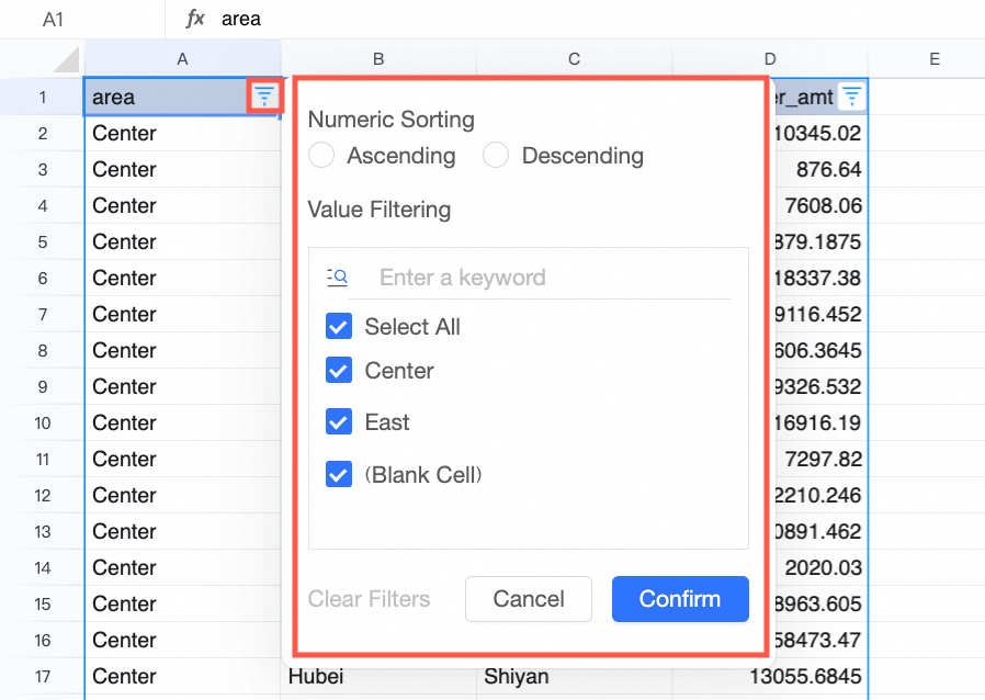
Filter | Allows you to filter data in the table and sort numerical values in ascending or descending order.
|
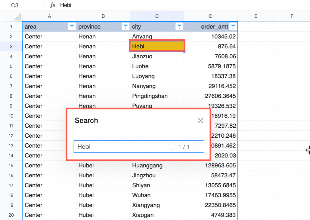
Search for data | Allows you to search for data by entering keywords.
|
View
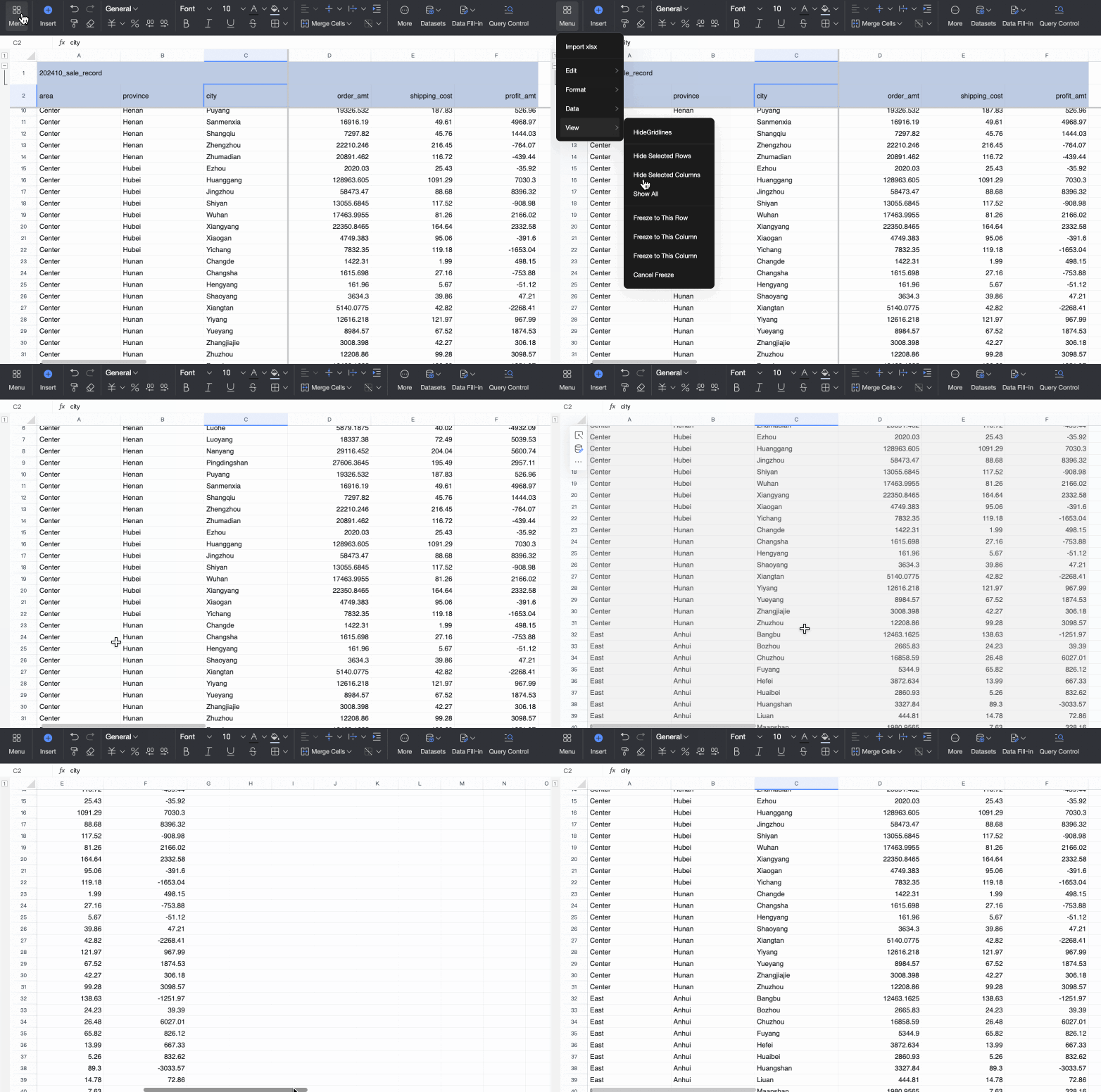
You can perform the following view-related operations.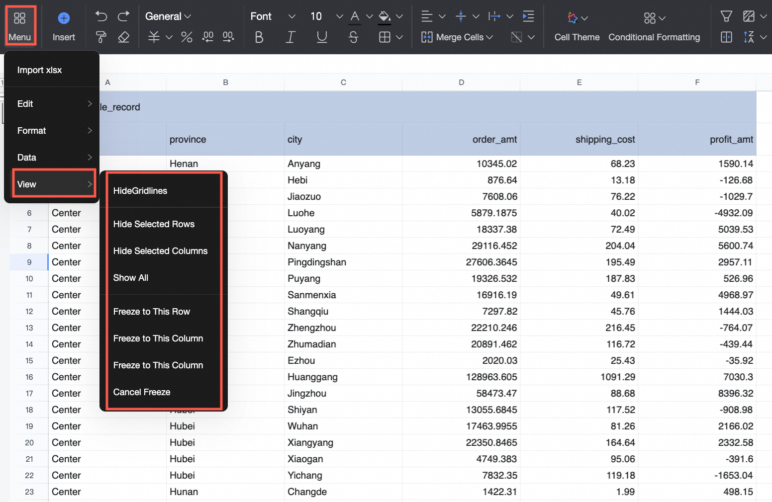
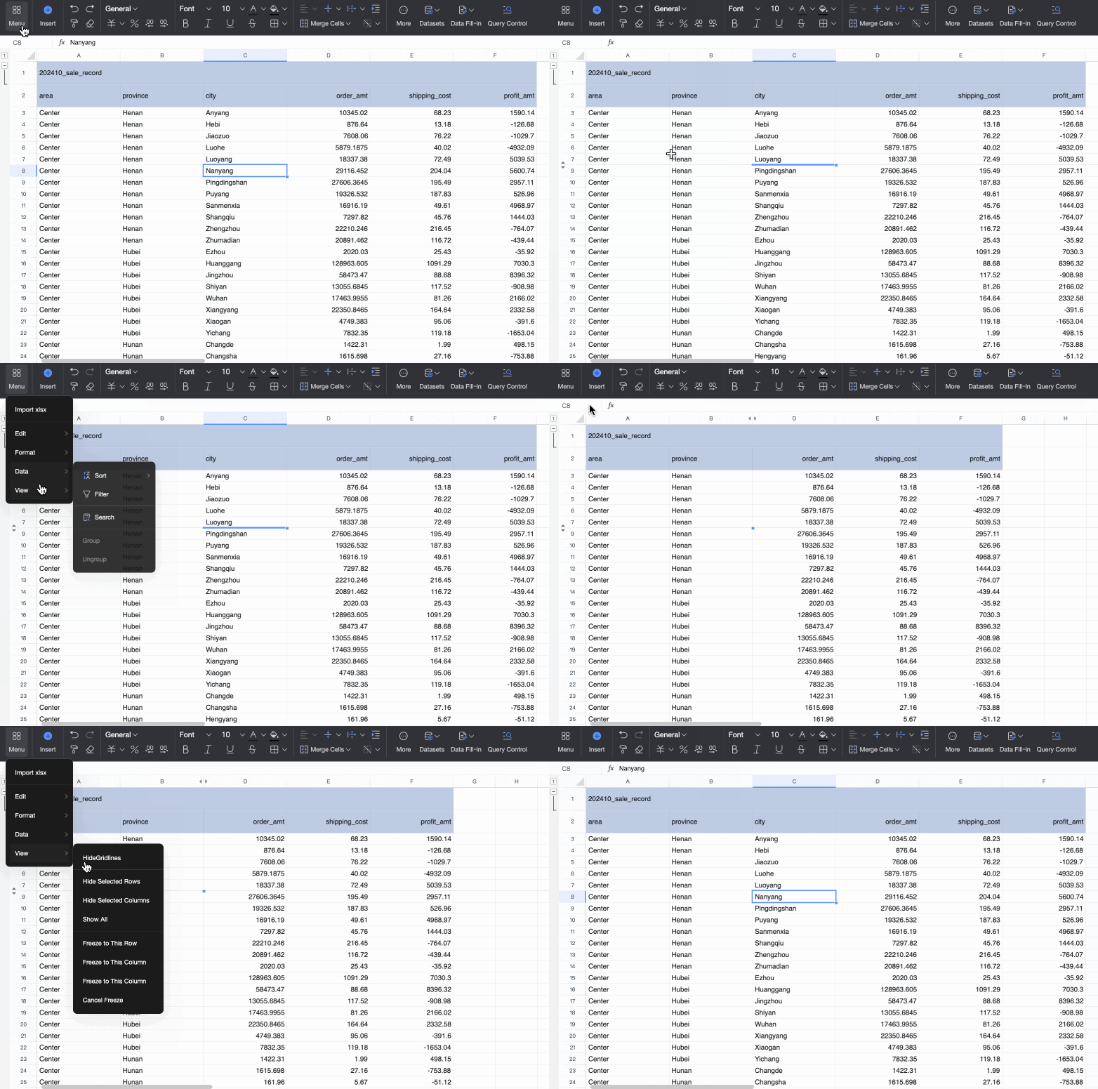
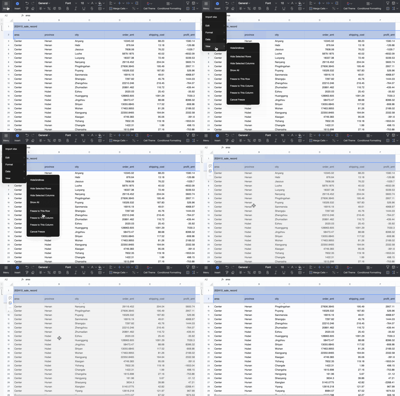
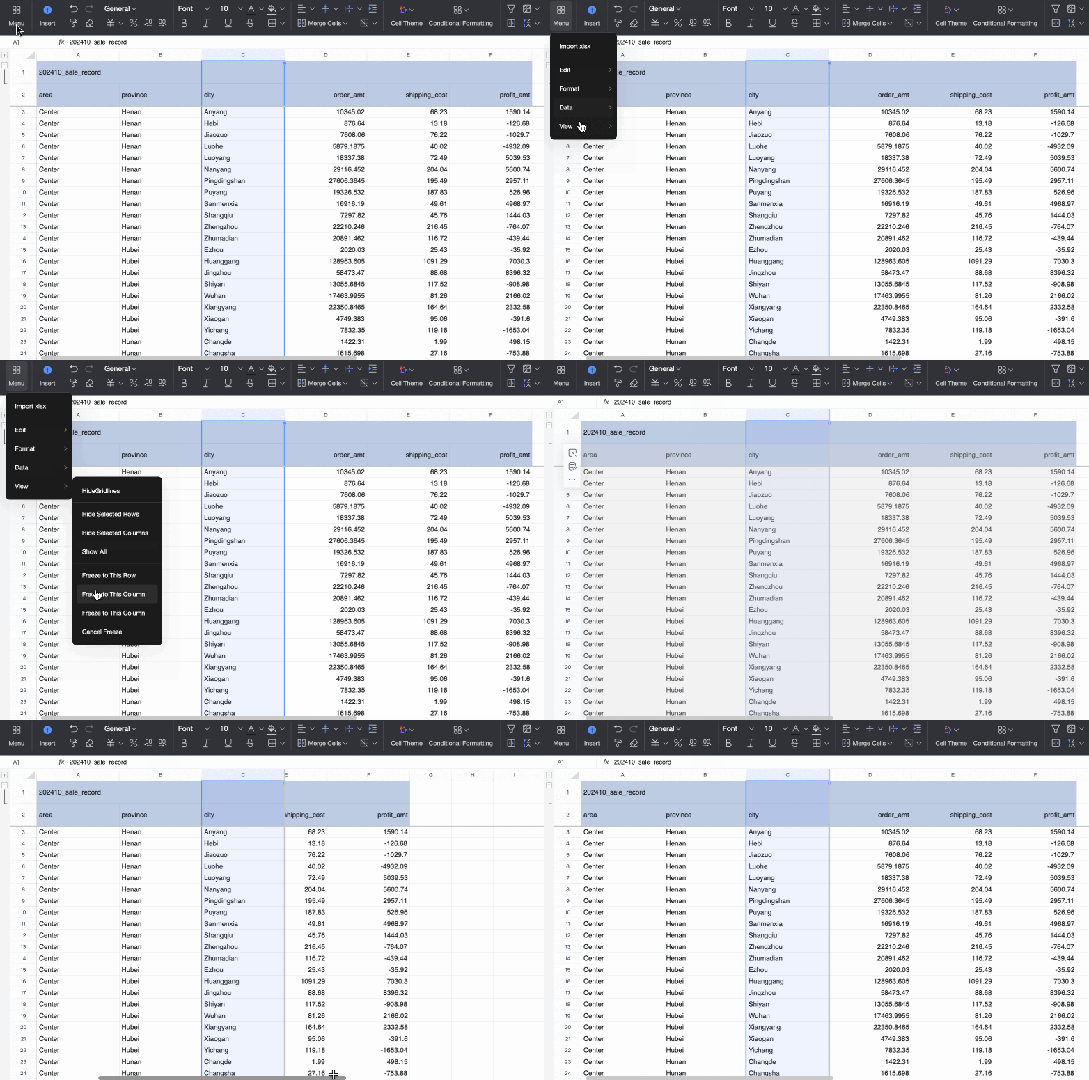
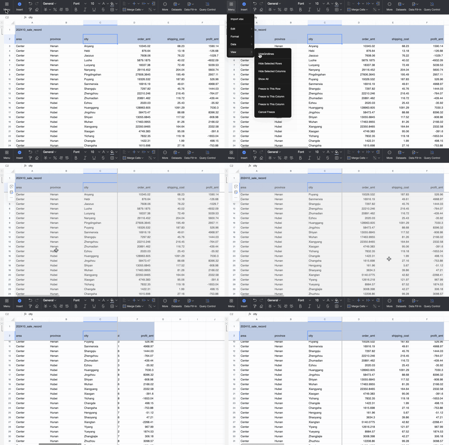
Option | Description |
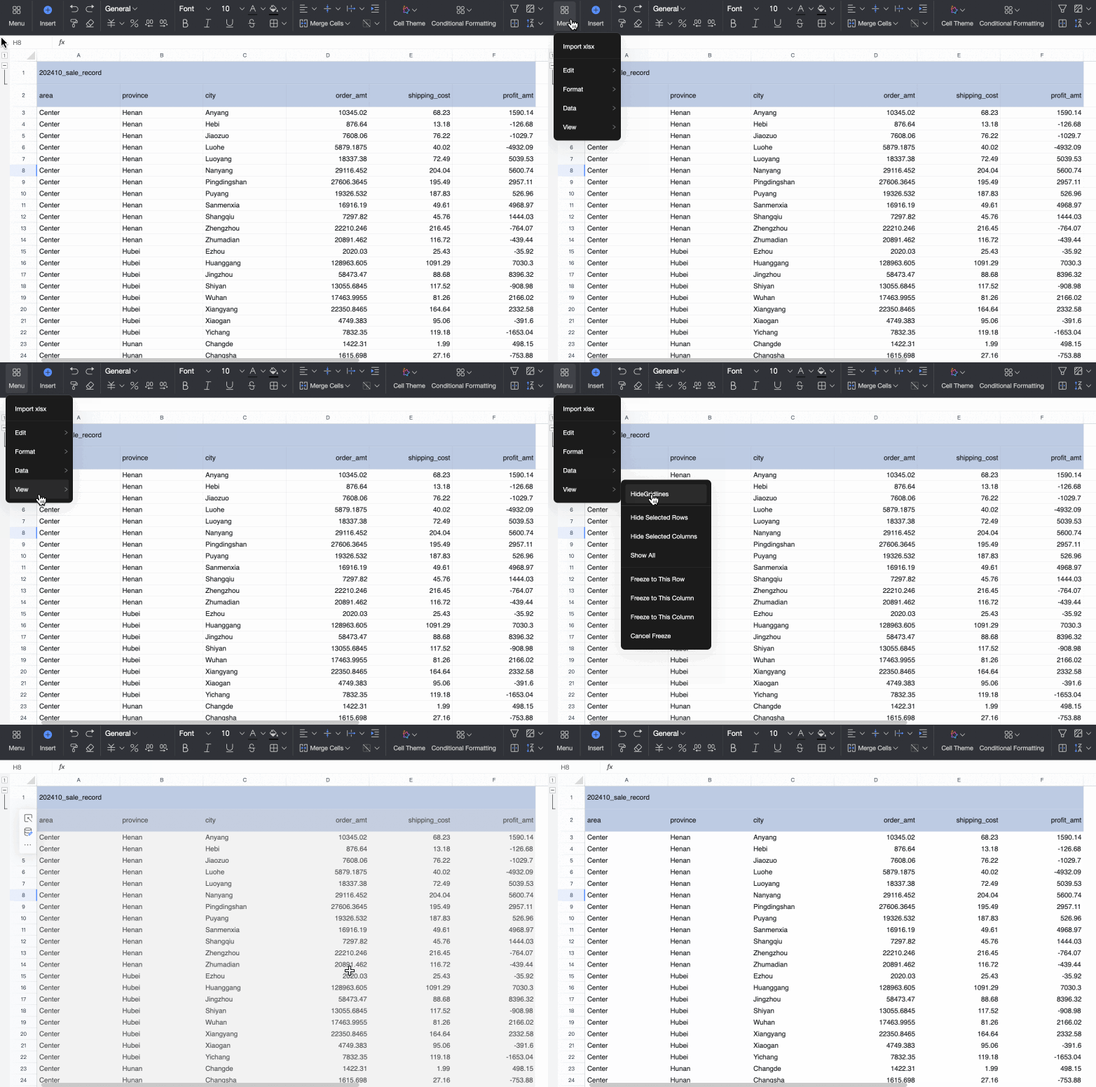
Hide/show gridlines | Show or hide gridlines.
Note The setting for hiding gridlines can be saved. |
Hide/unhide selected rows/columns | Hide or unhide selected rows or columns.
|
Freeze to current row | Keeps the current row visible while you scroll through the rest of the sheet.
|
Freeze to current column | Keeps the current column visible while you scroll through the rest of the sheet.
|
Freeze to current row and column | Keeps both the current row and column visible while you scroll.
|
Unfreeze | Unlocks all rows and columns so you can scroll through the entire sheet.
|
Toolbar
You can use the toolbar to perform the following operations on the data in a workbook:

① Undo, Redo, Format Painter, and Clear Formats.
② Set data format.
③ Set text format.
④ Set cell style (such as fill color and merge cells).
⑥ Set conditional formatting.
⑦ Set filter, sort, freeze, and create pagination.
⑧ Create a card view.
⑨ More functions (pivot table, Image, drop-down list, Hyperlink, Comment, block alignment, and Search).
⑩ Insert a dataset, which supports inserting a dataset table and a freestyle cell. For more information, see Create a workbook.
⑪ Set up data entry.
⑫ Add a query control.
⑬ Use AI functions.
Sheet settings
You can configure the sheets in your workbook as follows.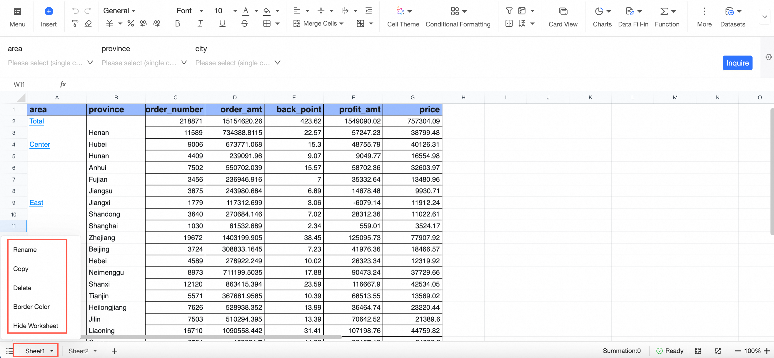
Option | Description |
Rename | Rename the current sheet. Note Sheet names can contain spaces, but cannot consist only of spaces. |
Copy | Duplicates the current sheet, including its blocks, formatting, functions, and data source connections. |
Delete | Delete the current sheet. |
Border color | Set the border color for the current sheet tab.
|
Hide sheet | Hide the current sheet. |
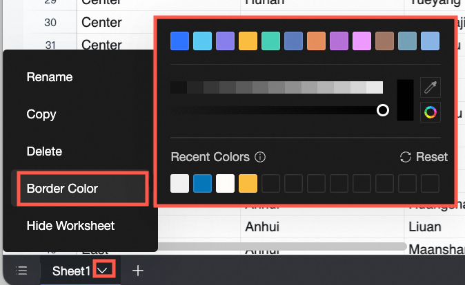
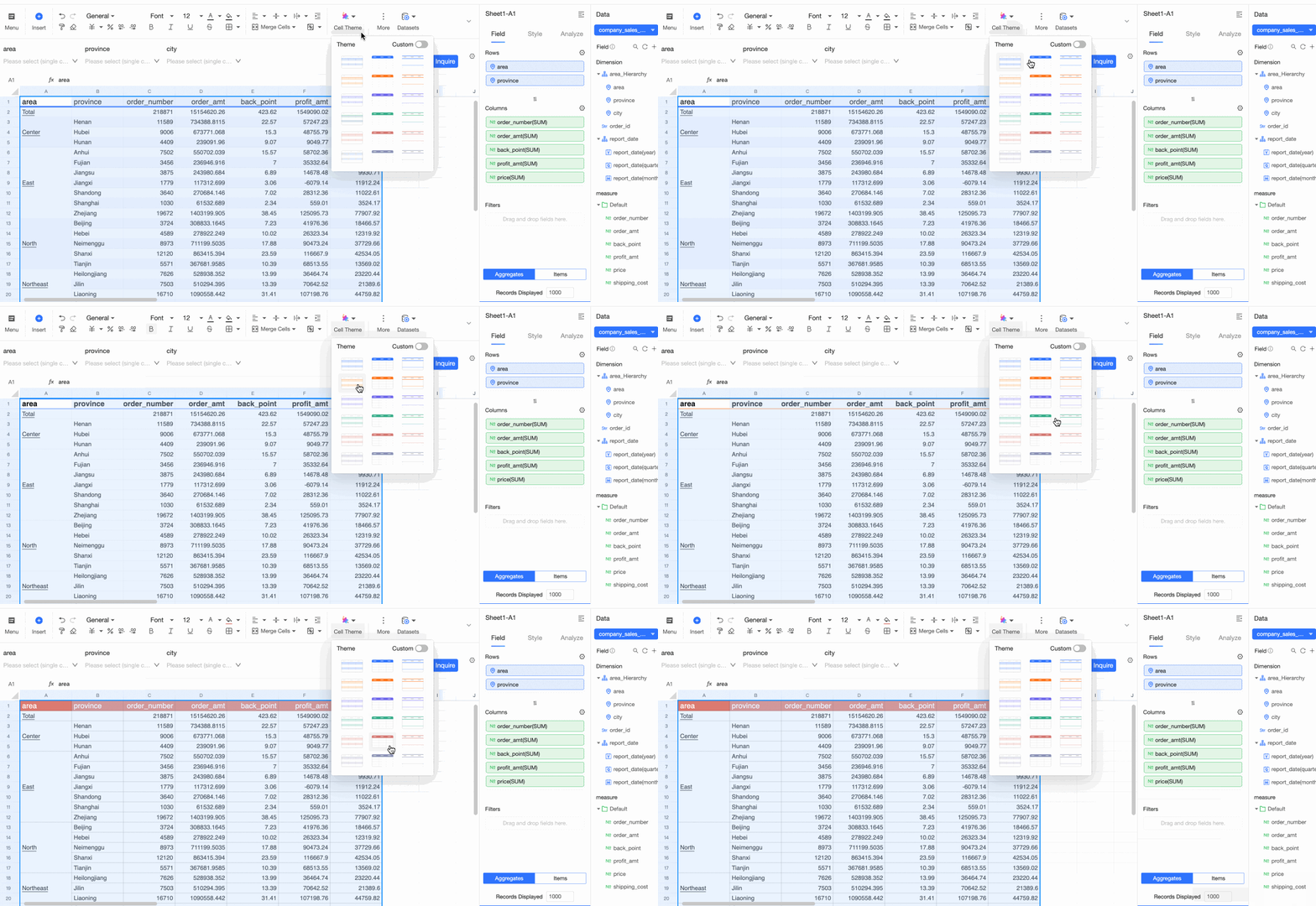
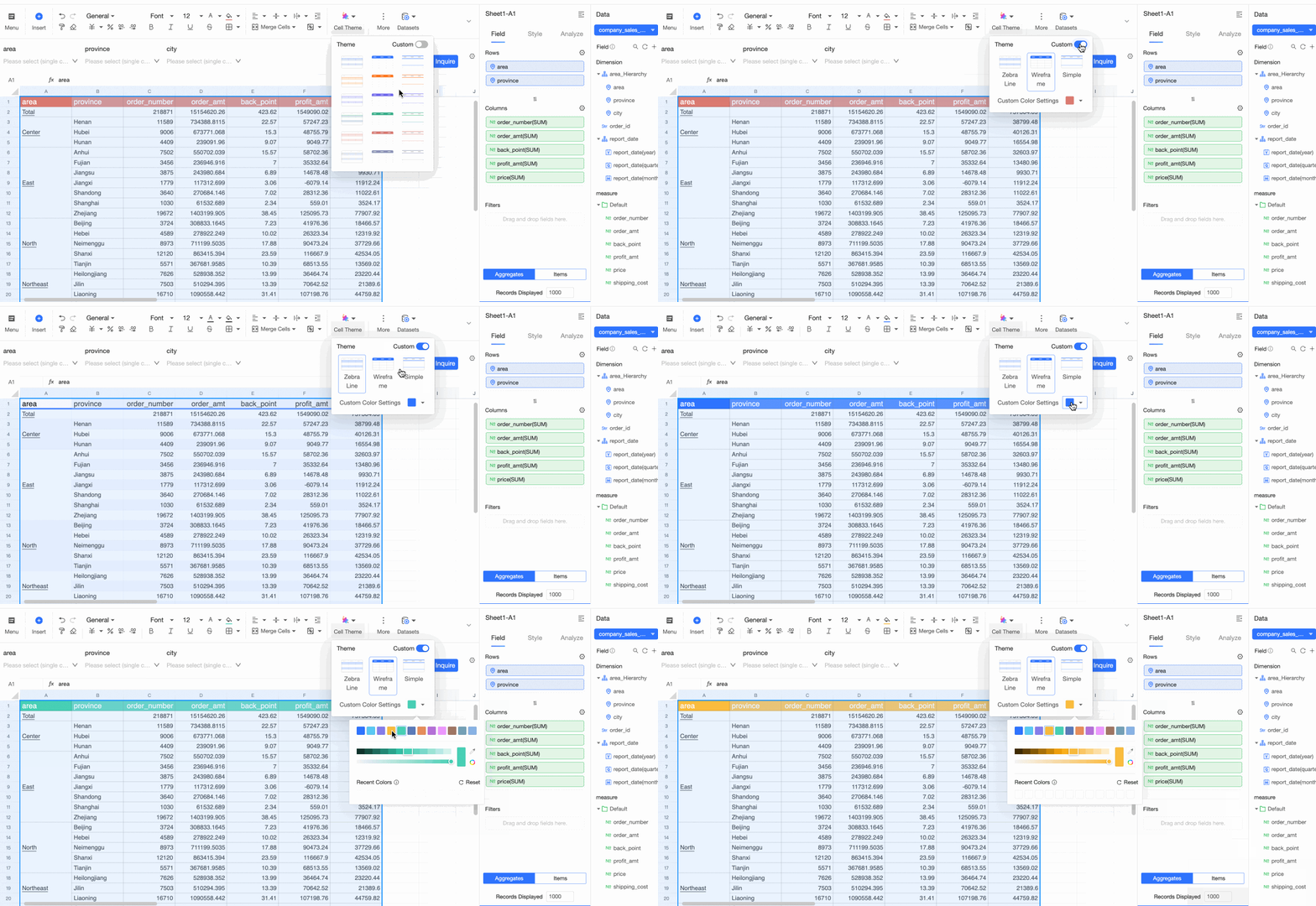
Cell themes
You can apply built-in system themes.
You can also set custom themes.
Conditional formatting
You can create rules to automatically format cells that meet specific conditions. Follow these steps:
Conditional formatting rule
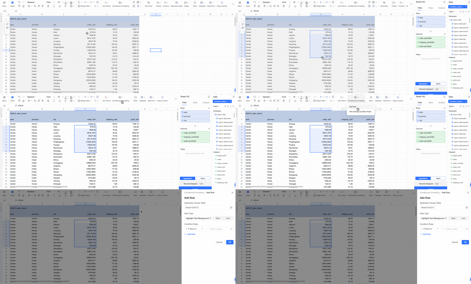
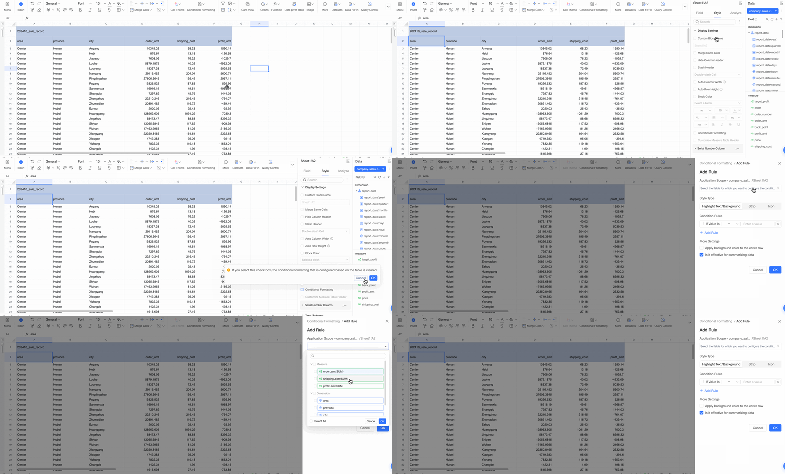
In the workbook, select the cell range or dataset field where you want to apply conditional formatting.
Area type
Instructions
Cell range
Select the desired range of cells directly in the table. Then, on the toolbar, click Conditional Formatting > Add Rule.
Dataset field
In the Style panel of the dataset, enable conditional formatting and select the fields to which you want to apply the rules.
In the Add Rule window, configure the rule details, including Style Type and Condition Rule.
Content
Description
Highlight Text/Background
Application: Create rules to highlight cell text or background colors, visually emphasizing key data to help readers quickly identify important information.
Instructions: Configure the calculation method for the rule (①), text and background colors (②), and text and cell border styles (③). You can use a custom formula for calculations. For details on using custom formulas, see Common applications of custom formulas.
More Settings: When applying conditional formatting to a dataset field, you can quickly apply a configured background color rule to the entire row and choose whether it affects summary data.
Data bars
Application: Represent numerical values with colored bars of varying lengths to visually show the relative size or comparison of data.
Instructions: Configure the minimum and maximum values (①), enable or disable a gradient effect for the data bars (②), and set colors for positive and negative values (③).
More Settings: When applying conditional formatting to a dataset field, you can choose whether it affects summary data.
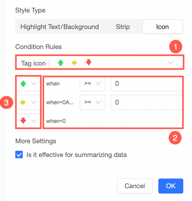
Icons
Application: Display specific icons in cells based on value comparisons to clearly show the relationship between current data and target data, thereby visualizing data trends.
Instructions: Select an icon set style (①), set comparison rules and target values (②), or customize the icon for each rule (③).
More Settings: When applying conditional formatting to a dataset field, you can choose whether it affects summary data.
Color scales
Application: Apply a color gradient to the background of cells based on their values. This helps to clearly show data distribution and trends, allowing viewers to quickly identify minimum, maximum, and intermediate values.
Instructions: Select a color scale style (①), define the criteria for minimum, midpoint, and maximum values, and set the corresponding cell fill colors (②).
More Settings: When applying conditional formatting to a dataset field, you can choose whether it affects summary data.
(Optional) In the Conditional Formatting window, you can view the created conditional rules, as well as edit, delete, or add them.




Custom formula applications
When you select Highlight Text/Background as the style type, you can set the condition rule to Custom Formula. This allows you to enter a formula that fits your business logic. The following examples use a company sales revenue table to demonstrate common scenarios.
Keep the following points in mind when writing custom formulas:
Before writing the formula, ensure you have selected the cell range or dataset field for the conditional format. For example, in the following scenarios, the cell range for the revenue column (such as I3:I7) must be selected.
Formulas should typically start with an equals sign (
=) and must return a boolean value of TRUE or FALSE (or their numerical equivalents, 1 or 0). The specified format is applied if the formula returns TRUE.Depending on your needs, use relative references (e.g.,
A1) or absolute references (e.g.,$A$1) to correctly refer to cells or ranges. A relative reference adjusts automatically when the formula is applied to different cells, while an absolute reference always points to the same cell.
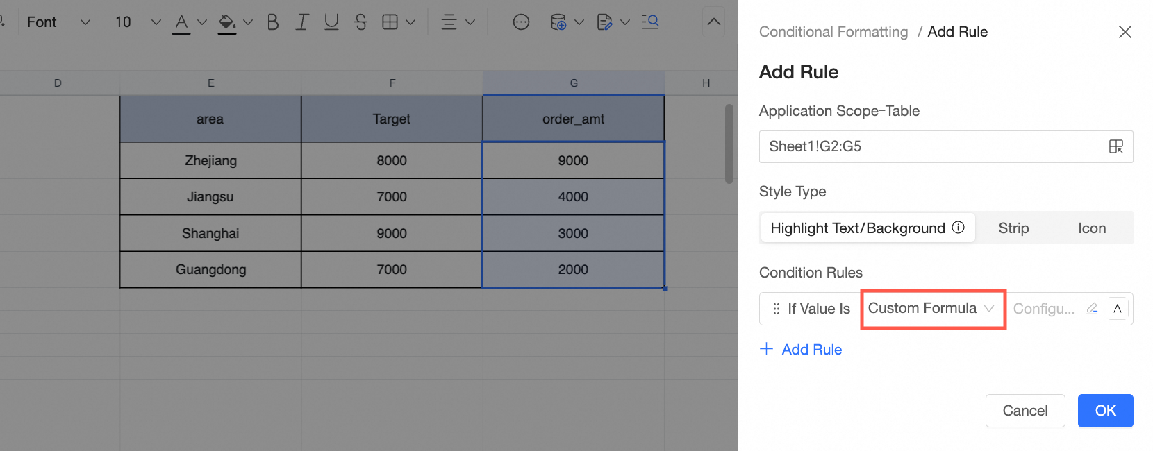
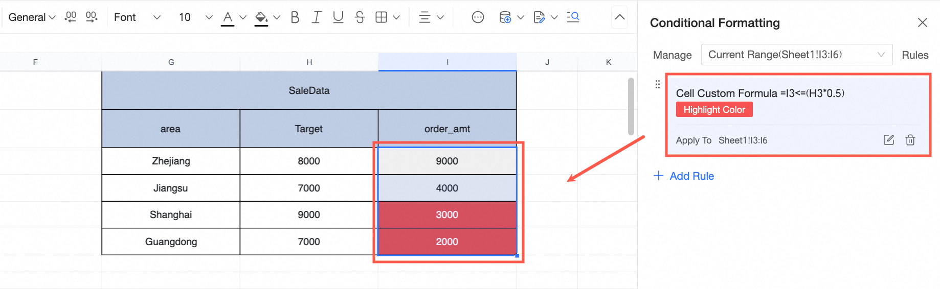
Scenario 1: Compare with another cell
Highlight the revenue cell if the revenue is less than 50% of the target revenue.
Formula:
=I3<=(H3*0.5)Explanation: This formula uses a standard comparison. Since the cell references need to adjust for each row, relative references are used. You only need to write the rule for the first row of data.
Result: After you enter the custom formula and set the cell text and background colors, click OK. The conditional format is applied to the selected cell range.
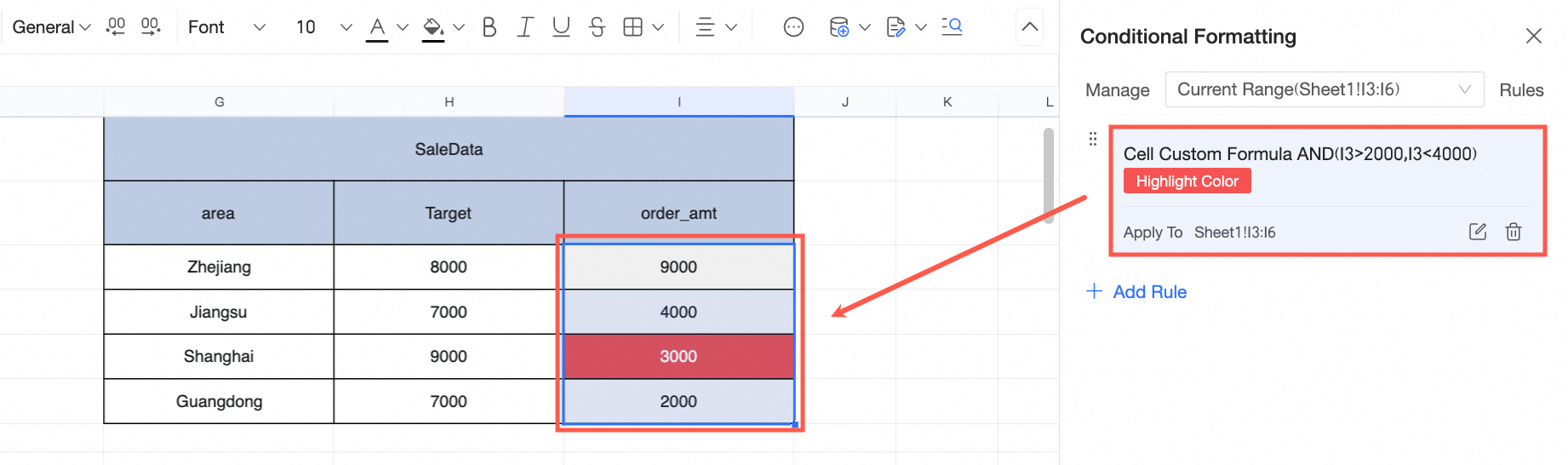
Scenario 2: Evaluate its own value
Highlight the revenue cell if the revenue is greater than 20 million and less than 40 million.
Formula:
=AND(I3>2000,I3<4000)Explanation: The AND function is used to define multiple logical conditions. Relative references are used so that the rule applies correctly to each row in the selected range.
Result: After you enter the custom formula and set the cell text and background colors, click OK. The conditional format is applied to the selected cell range.
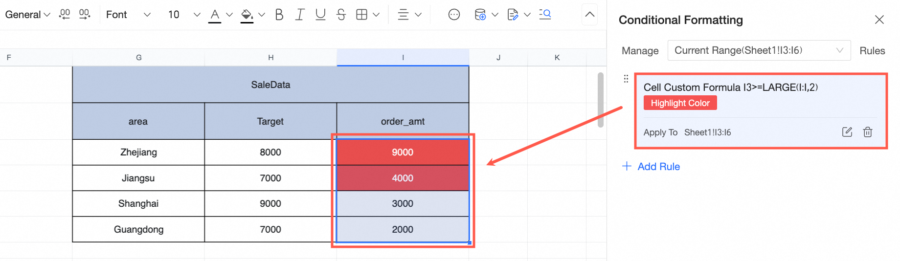
Scenario 3: Find top or bottom N values
Highlight the cells for the top 2 revenue amounts.
Formula:
=I3>=LARGE(I:I,2)Explanation: The LARGE function finds the 2nd largest value in column I (the revenue column). Any cell value in column I that is greater than or equal to this value is considered to be in the Top 2. Relative references are used to evaluate the rule for each row.
Result: After you enter the custom formula and set the cell text and background colors, click OK. The conditional format is applied to the selected cell range.
Sort
Supports ascending, descending, and custom sorting.
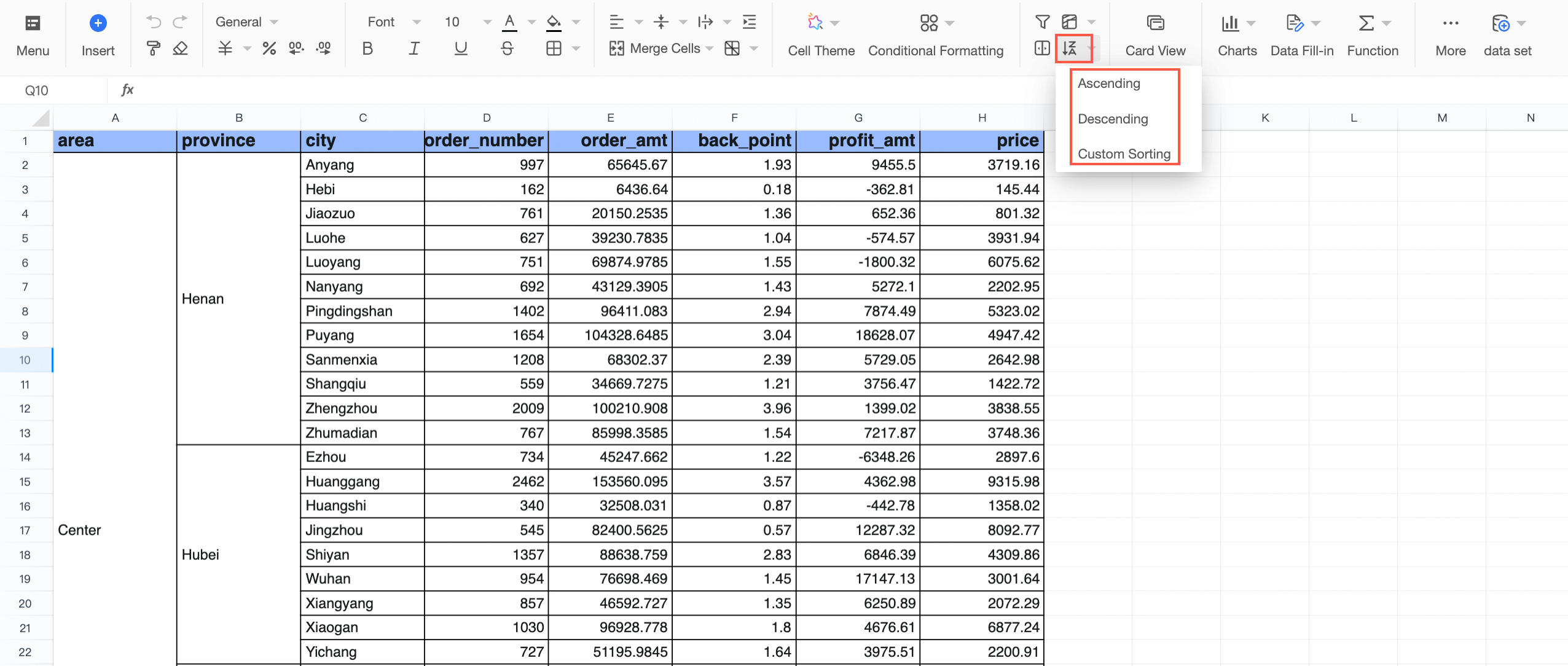
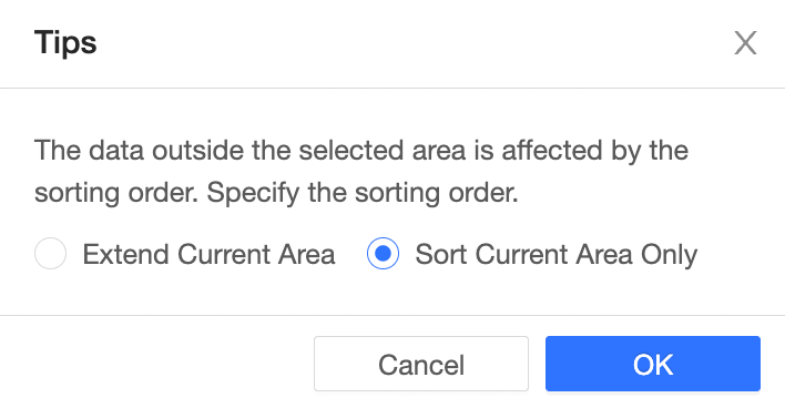
For ascending and descending sorts, you can choose to expand the selection or sort only the current selection.
NoteExpanding the selection is not supported for ranges that contain vertically merged cells. To sort an expanded selection, unmerge the cells first.
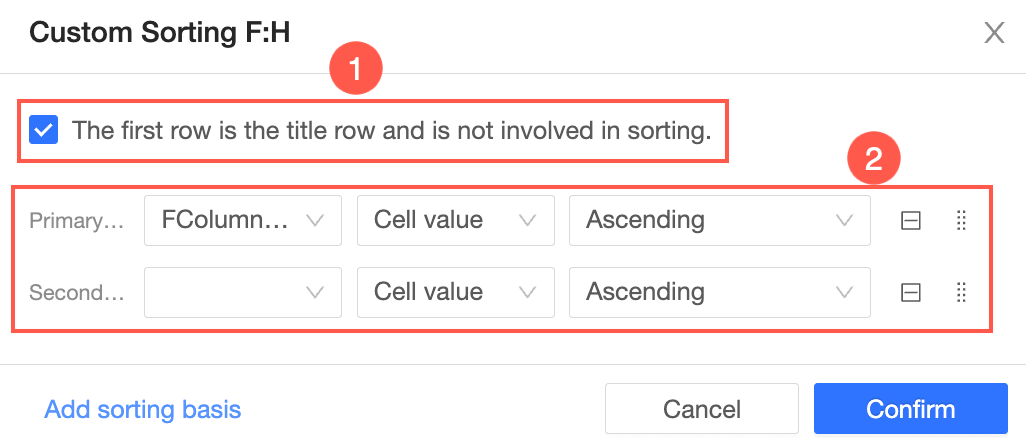
Custom sort
① You can choose whether the first row is included in the sort. If selected, the first row is treated as a header and not sorted.
② Set a primary sort key and add multiple secondary keys. You can drag to reorder the sort keys.
Pagination
Click the
icon on the toolbar to configure pagination.Parameter
Description
Select dataset
Select the dataset for which to create pagination.
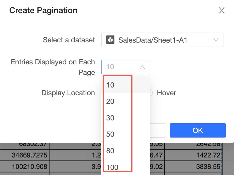
Rows per page
Set the number of rows to display per page. Options are 10, 20, 30, 50, 80, and 100.
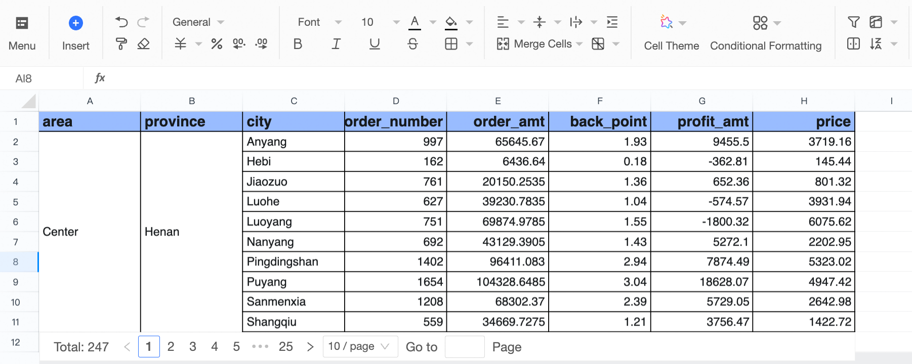
Display position
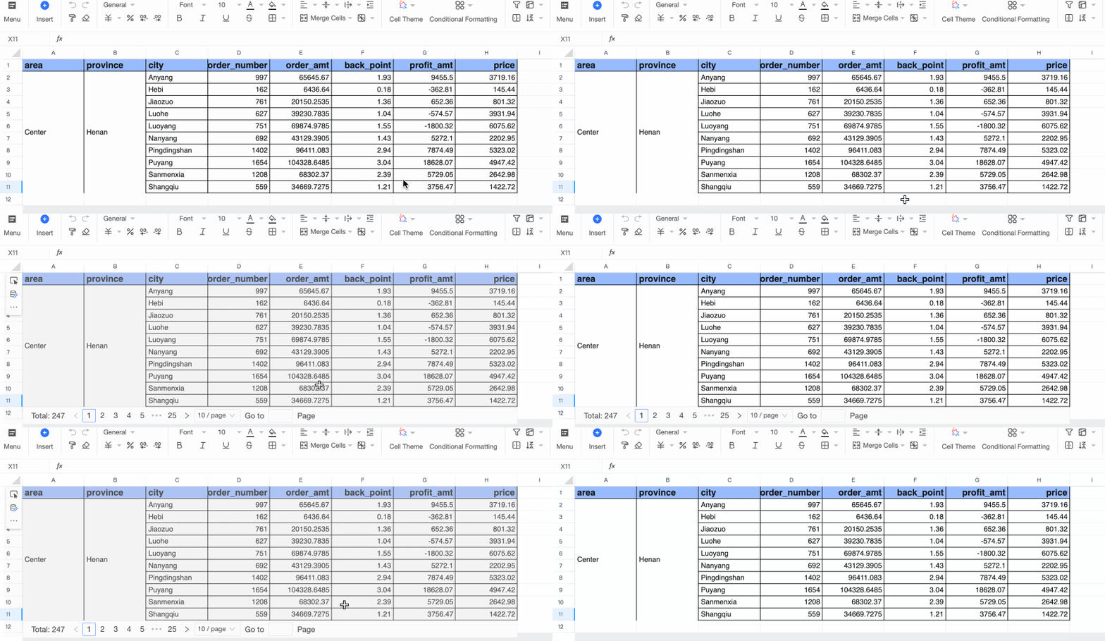
Set the display to Always show or Show on hover.
Always show effect:
Show on hover effect:
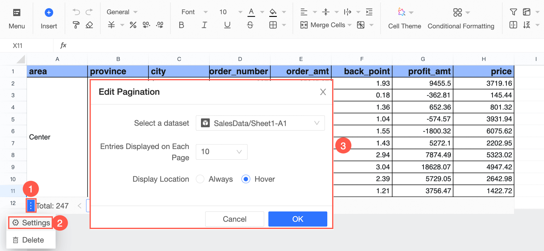
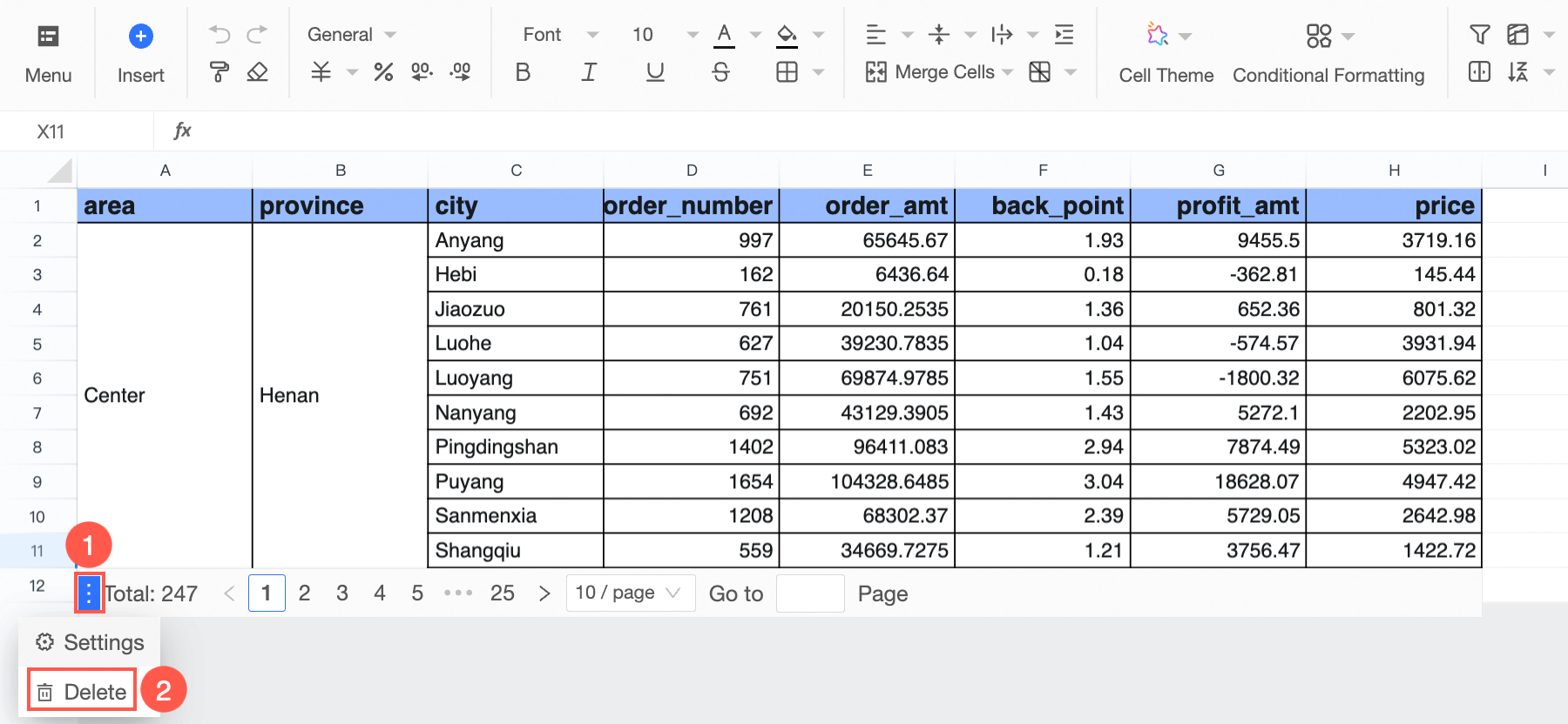
You can edit the paginator as shown in the figure.
You can also delete the paginator as shown in the figure.
 icon on the toolbar to configure pagination.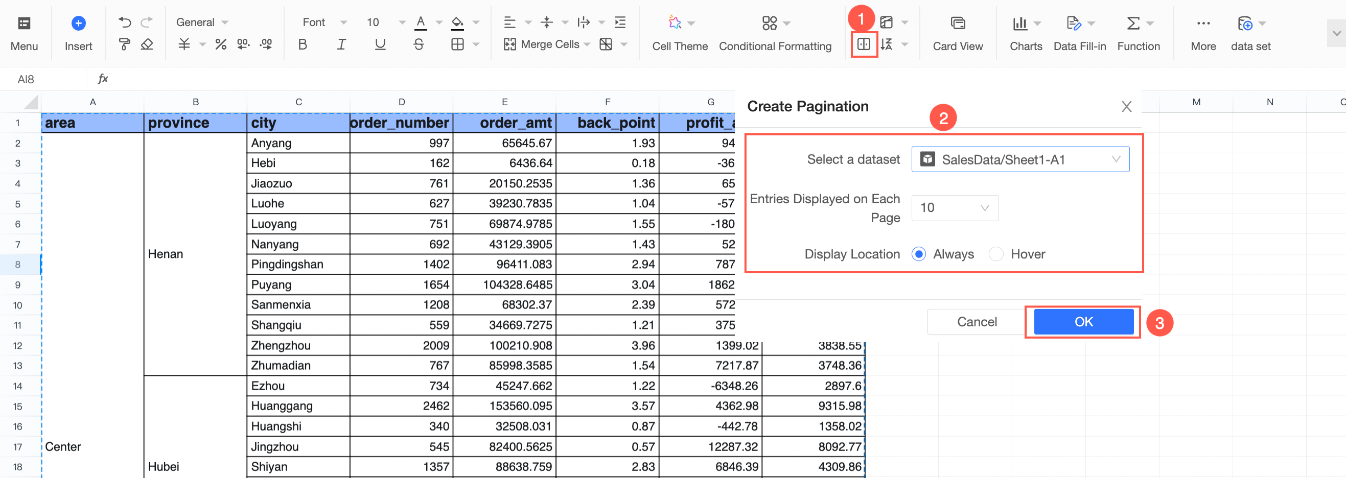
Insert a drop-down list
A drop-down list can be used to quickly filter and populate categories. Follow these steps to add a drop-down list:
① On the workbook editing toolbar, click Drop-down list.
② On the Drop-down list settings page, add labels for the data items.
③ Click OK.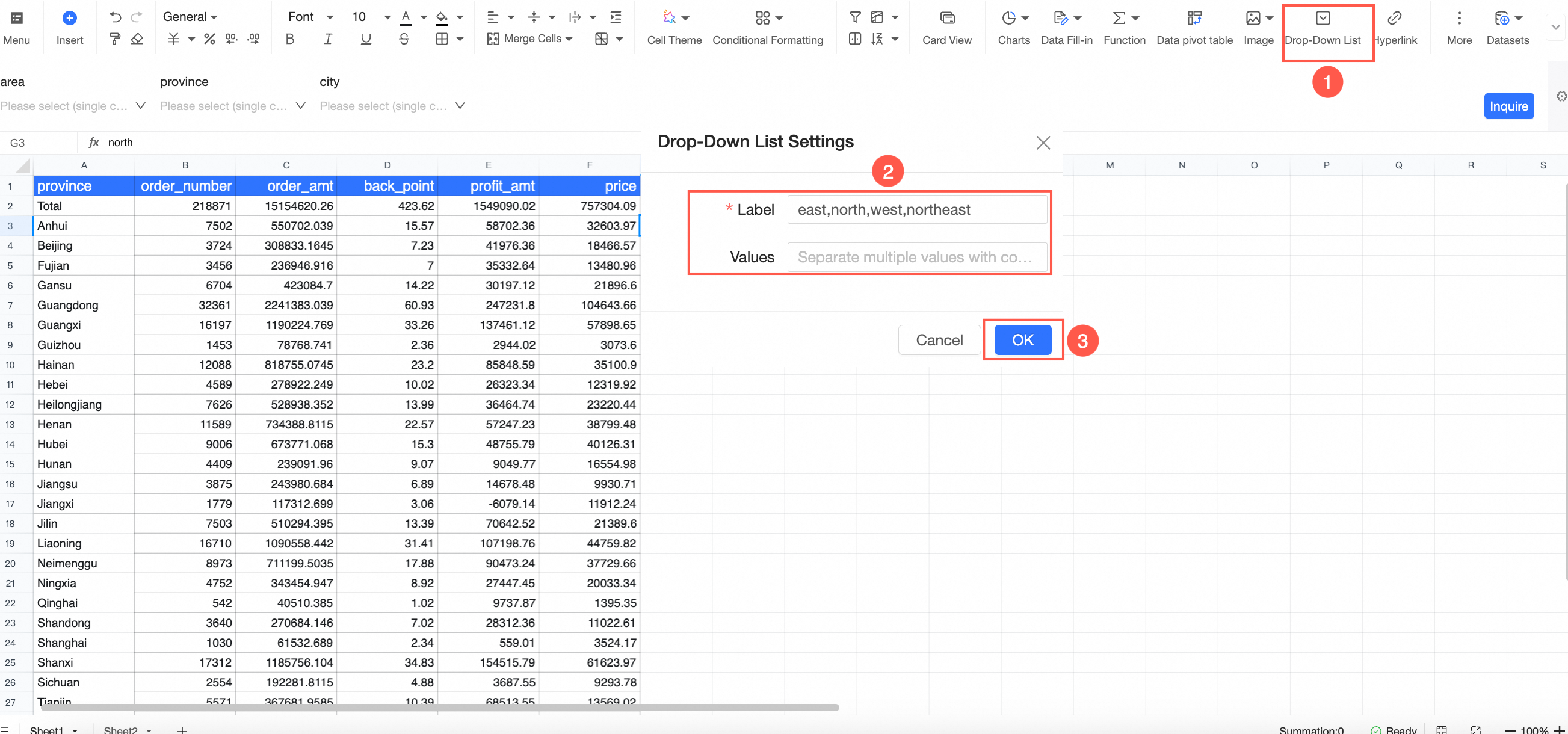
The effect is as follows:
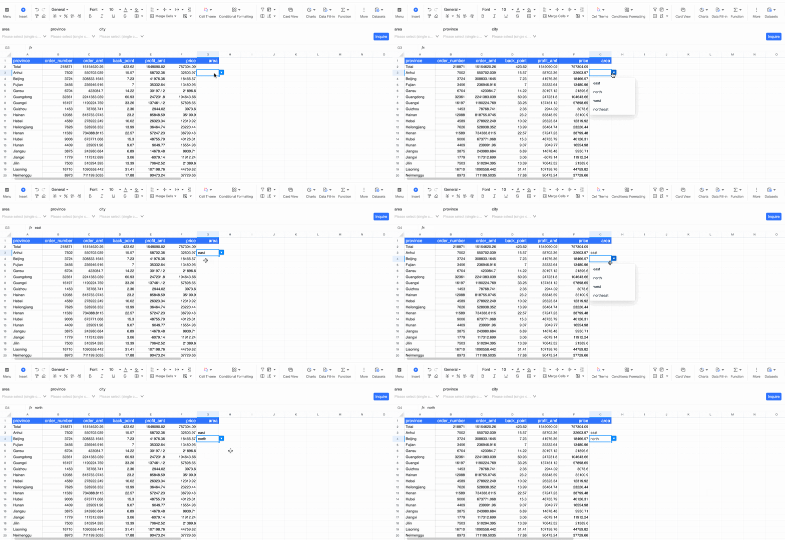
Separate multiple labels with commas (,).
If the message "This operation is not allowed because it may affect the data of nearby datasets." appears, copy the content to another area of the workbook and then try the operation again.
Block alignment
In many business scenarios, data for a single domain is spread across multiple datasets. To display this related data on one sheet, you may need to combine blocks from different datasets. You can use block alignment to match different blocks based on alignment rules. After alignment, the values displayed in the reference block remain unchanged. The row order and content in the matching blocks are adjusted to align with the reference block. This gives you a cleaner layout.
Example use case: Assume you have two datasets. Dataset A contains some employees' names, employee IDs, departments, and ages. Dataset B contains all employees' IDs and performance scores. You want to show names, IDs, and departments from dataset A, along with the corresponding performance scores from dataset B, on the same sheet.
First, insert both datasets into the sheet by using a dataset table (as shown on the left). Block A contains employee name, ID, and department from dataset A. Block B contains employee ID and performance score from dataset B.
After the data loads, you may notice a problem: data in the same row in block A and block B may not belong to the same employee. Also, block B contains more employees than block A, but you only care about employees that exist in dataset A.
Use block alignment to fix this. Use the employee ID in block A to find the matching records in block B. Then place the scores in the corresponding rows and remove extra rows that do not exist in block A. The result is shown on the right.

On the workbook editing page, choose More > Block alignment on the toolbar.
You can also go to the dataset table configuration panel and choose Analysis > Advanced configuration. Click the
icon to the right of Cross-block alignment configuration.In the Cross-block alignment configuration dialog box, select the sheet (①). The available dataset blocks (②) change with the selected sheet.
NoteYou can select only sheets that are not hidden.
You can select only dataset blocks that have row dimensions configured.
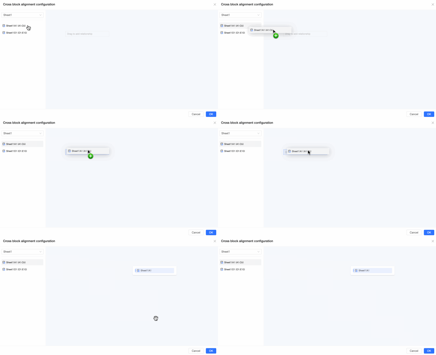
Select the target dataset block and drag it onto the canvas. In this example, first drag block A (which is
Sheet1!A1[A1:C6]).Drag the dataset block you want to align. You can place it in one of the following areas.
Area 1: The new block becomes the base block for the existing block. The existing block will be aligned to the new block.
Area 2: The new block is not associated with any blocks already on the canvas. It becomes a new, independent base block.
Area 3: The new block becomes the matching block for the existing block. The new block will be aligned to the existing block.
NoteYou can configure alignment for a maximum of five blocks per sheet.
A maximum of three levels of alignment relationships are supported. This means an alignment chain can contain a maximum of three blocks.
In this example, block B is the matching block. Drag block B (that is,
Sheet1!E1[E1:F10]) into Area 3.Click the
icon on the connecting line between the blocks. In the Alignment rule matching area on the right, set the linking fields for the block alignment. In this example, select Employee ID as the common field for both the reference column and matching column.NoteIf the matching block has two or more dimension fields, you can add up to two alignment rules.
If you configure two rules and the first-level field values are the same, alignment uses the field in the second rule.
Click OK to complete the configuration. The content of Block B is now aligned with Block A, displaying the performance scores for the corresponding five employees. Extra data is automatically removed.
(Optional) Select the duplicate Employee ID column in block B, right-click, and choose Hide selected columns. This hides the duplicate column and gives you a cleaner table.

 icon to the right of Cross-block alignment configuration.


 icon on the connecting line between the blocks. In the Alignment rule matching area on the right, set the linking fields for the block alignment. In this example, select Employee ID as the common field for both the reference column and matching column.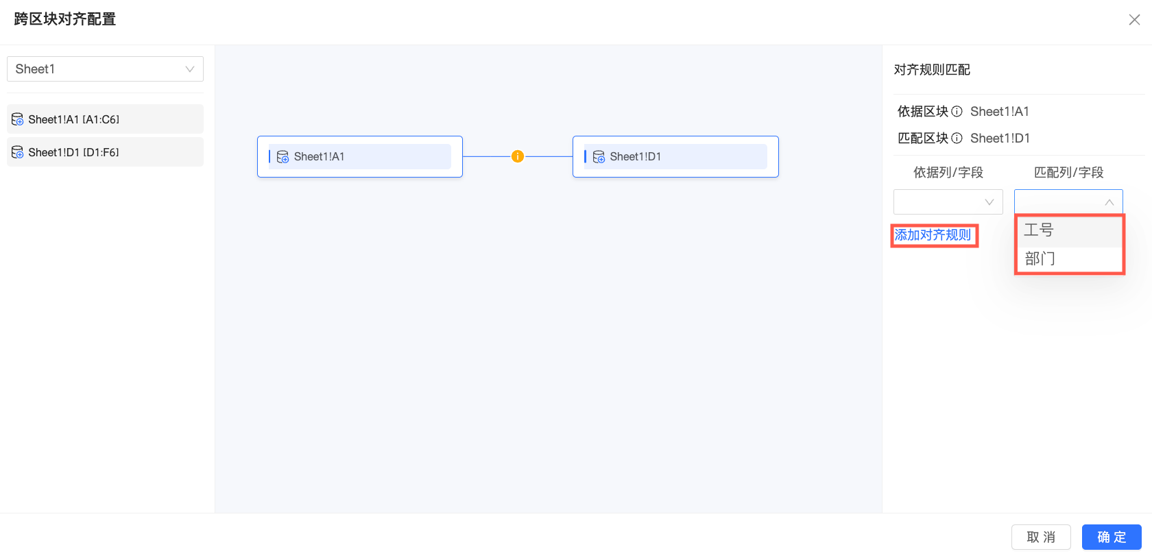


Insert a chart
You can insert charts into a workbook based on the data in the workbook. You can insert the following types of charts: line chart, column chart, pie chart, gauge, radar chart, scatter chart, funnel chart, and polar area chart.
In the data display section of a workbook, select a data range.
Insert a chart into the workbook.
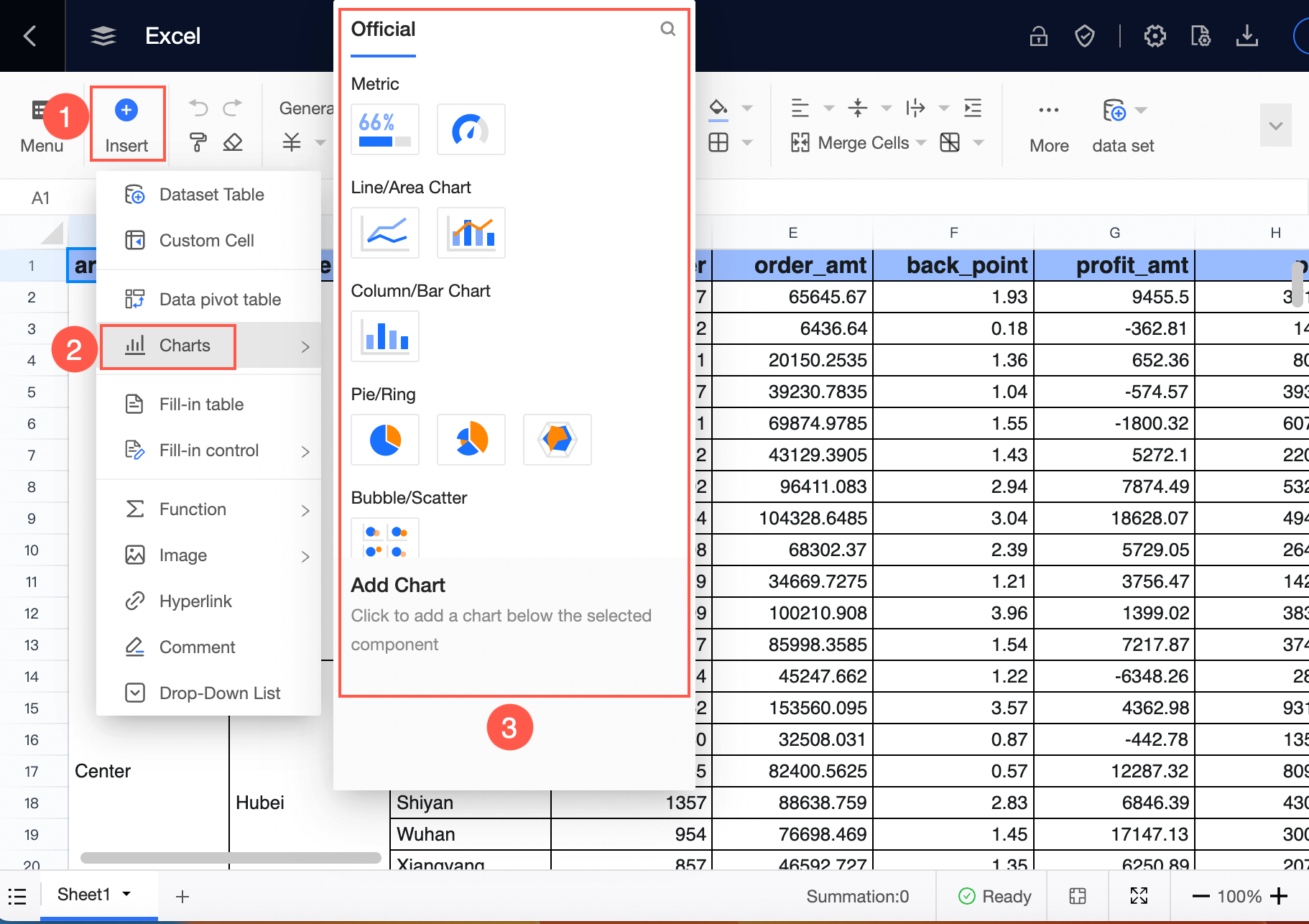
Method 1: Click ① Insert -> ② Charts -> ③ Select a chart.
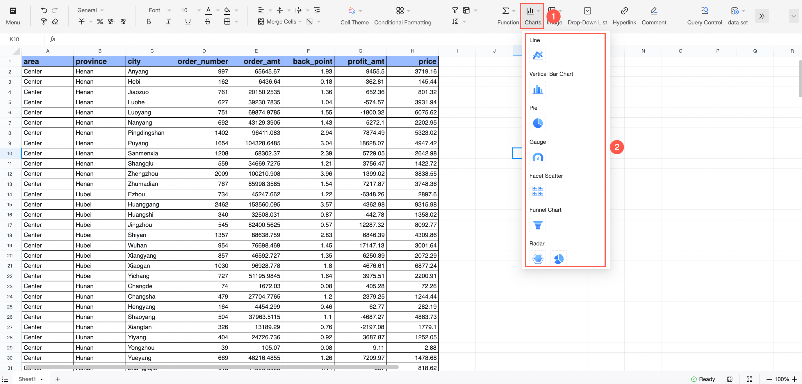
Method 2: ① Click the chart icon on the toolbar -> ② Select a chart.
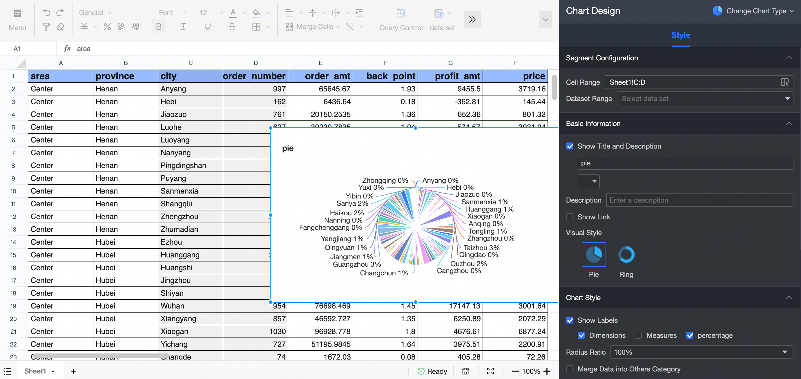
The chart is automatically displayed in the workbook. In the Chart Design panel on the right, you can configure the chart style.
In this example, a pie chart is selected.
For more information, see Overview of charts.
Pivot table
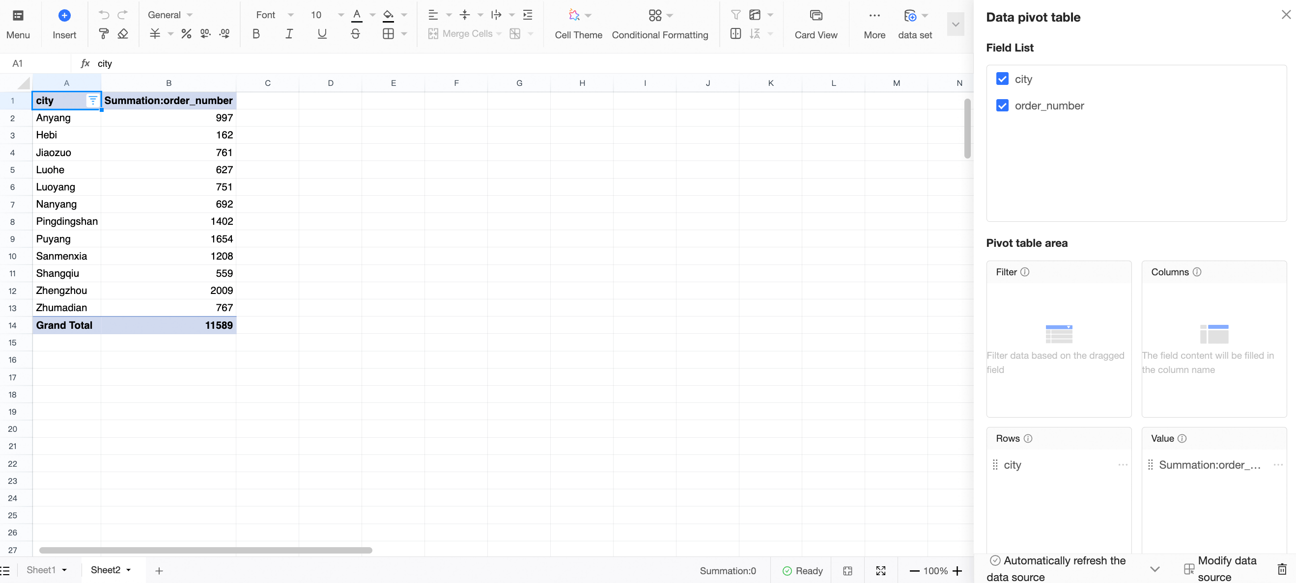
Pivot tables support Excel-like calculations, aggregation, and data analysis.
In the workbook display area, select a data range.
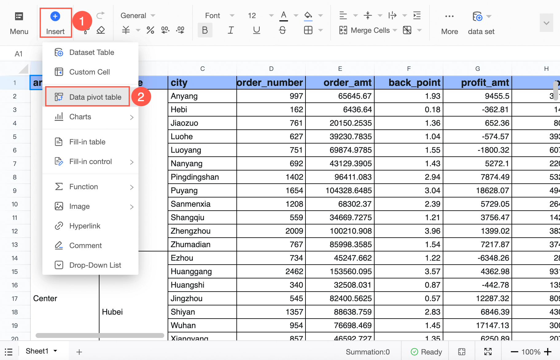
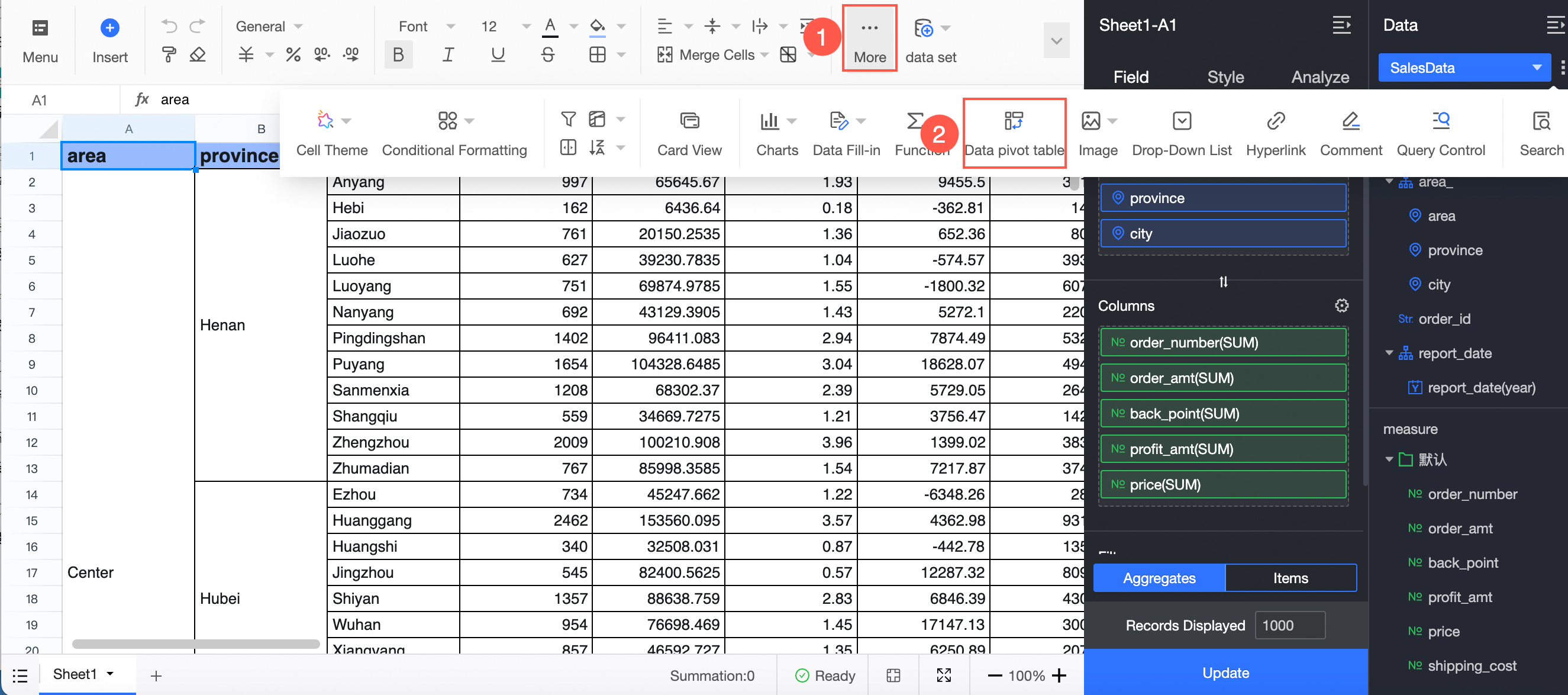
On the toolbar, create a pivot table as shown in the following figures.
Method 1: ① On the toolbar, click Menu -> ② Click Insert -> ③ Click Pivot table.
Method 2: ① On the toolbar, click More -> ② Click Pivot table.
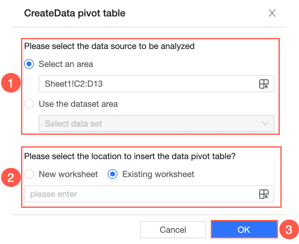
In the Create pivot table dialog box, you can configure the pivot table as shown in the figure.
① Select a range.
The range defaults to the one you selected in Step 1. You can modify the range directly in the input box or click the
icon to reselect a range.You can also select a dataset to create the pivot table.
② Choose where to place the pivot table.
You can place it in a new sheet or an existing sheet. For an existing sheet, you can enter the location directly or click the
icon to select a range.Click OK to create the pivot table.
You can then perform Excel-like calculations, aggregation, and data analysis.
 icon to reselect a range.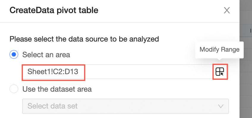
 icon to select a range.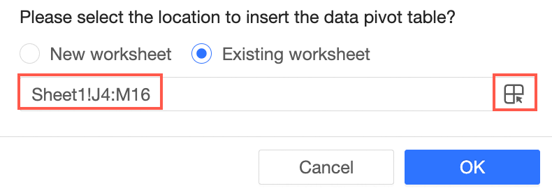
Right-click operations
Right-click in the workbook to access a context menu with options such as Cut, Copy, Paste, Insert rows and columns, Delete selected rows or columns, Clear, and Add comments.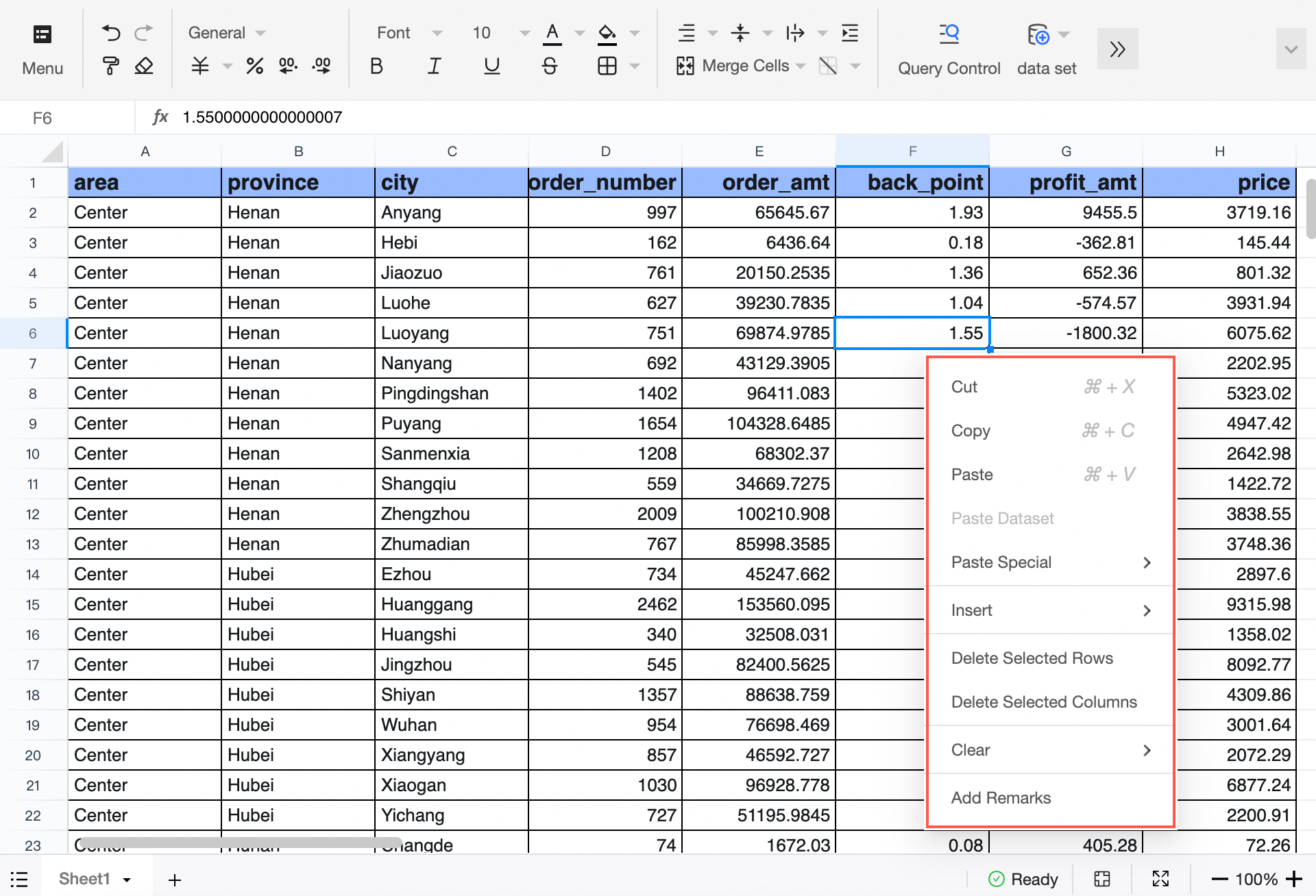
Option | Description |
Cut/Copy/Paste | Cut, copy, or paste data in the current cell. |
Paste special | Allows you to paste only values, only formats, or only formulas. |
Insert rows and columns | Insert rows above or below, or insert columns to the left or right. |
Delete selected rows or columns | Delete the rows or columns of the selected data. |
Clear | Clear all, content, formats, or comments. |
Add comment | Add a comment to a specific value.
|
Preview
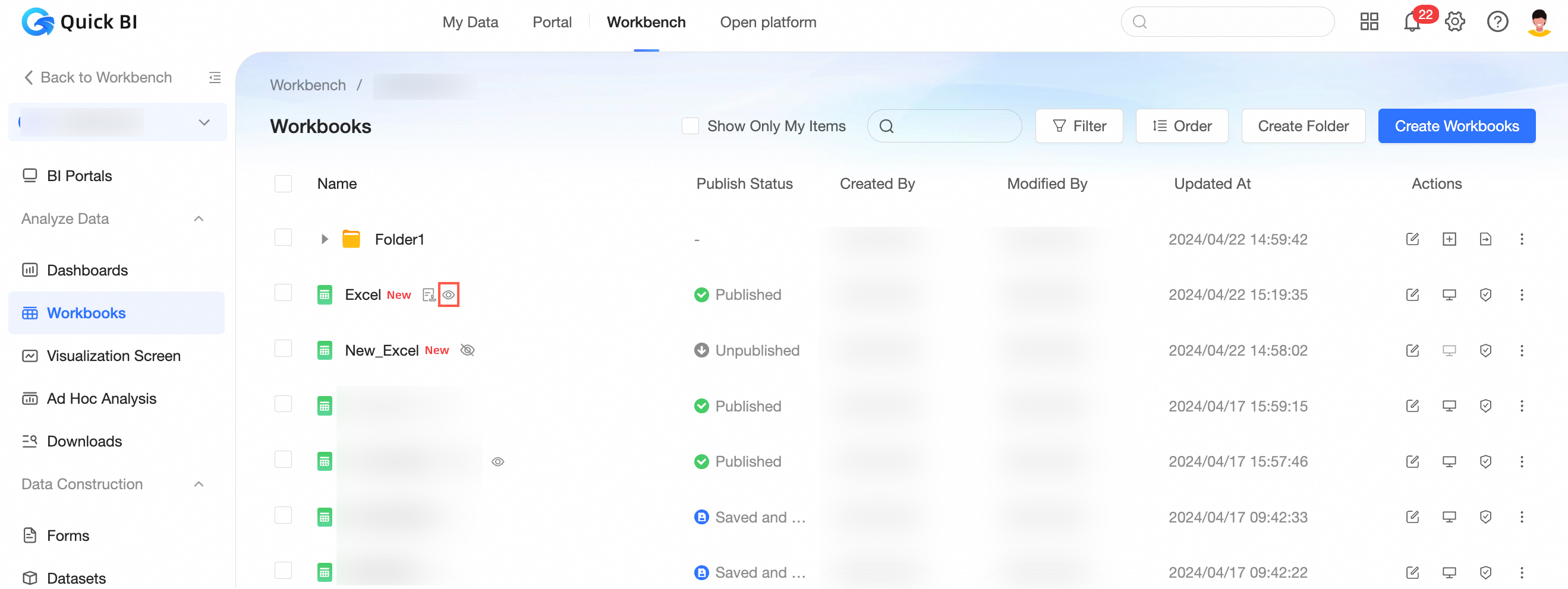
After publishing the workbook, you can click the  icon to preview it.
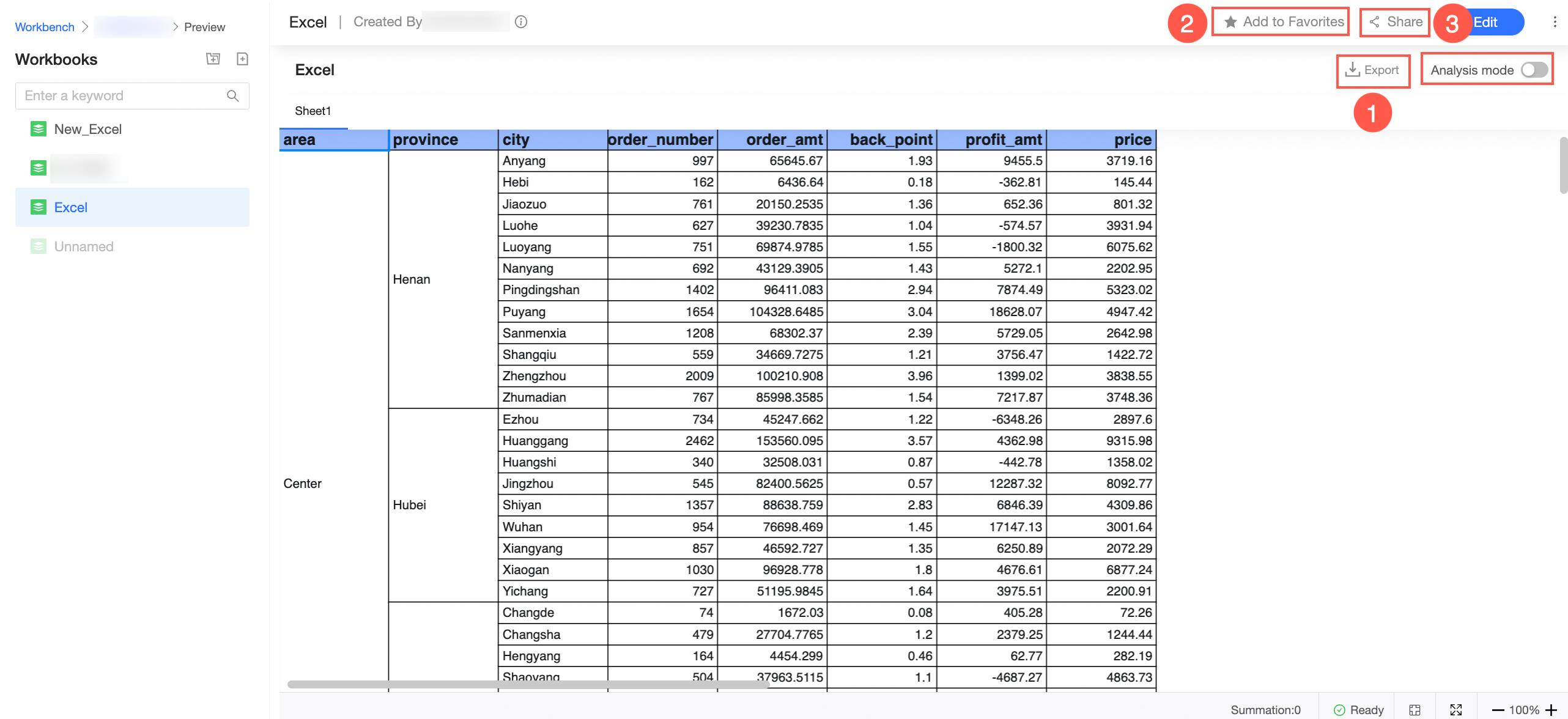
When previewing a workbook, you can turn analysis mode on or off.
Analysis mode off
When Analysis mode is off, selection borders are automatically hidden. You can export, add to favorites, and share. Additionally, if you need to display table row numbers and column headers on the preview page, you can go to the Page Settings on the table editing page and select the Show Row Numbers and Column Headers setting.
You can also click Edit to enter Edit mode.
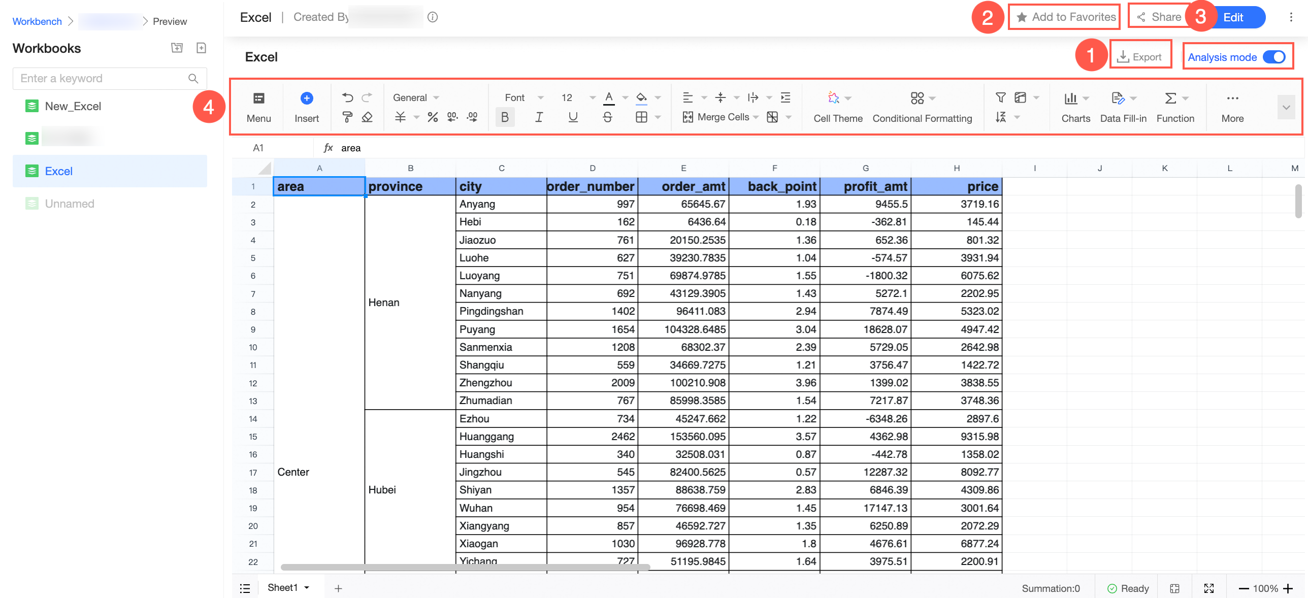
Analysis mode on
When Analysis Mode is enabled, in addition to exporting, adding to favorites, and sharing, the spreadsheet toolbar is displayed, and you can perform operations on the spreadsheet by using the menu and toolbar.
Light and dark modes
Go to the workbook page.
On the workbook editing page, click the
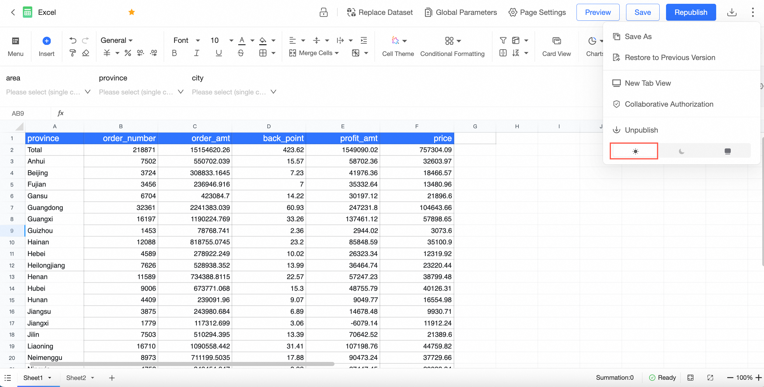
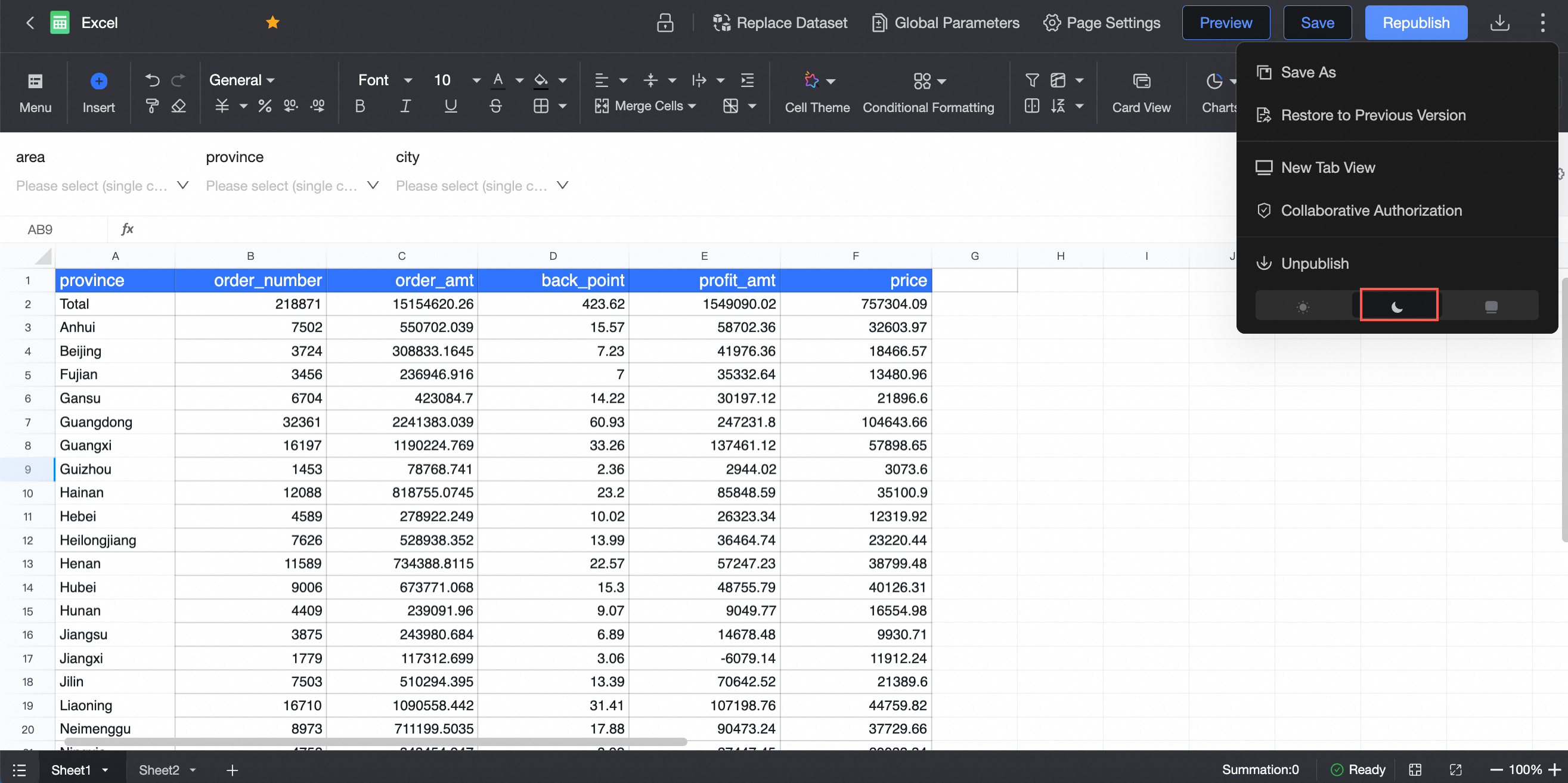
icon in the upper-right corner and find the mode switching icon at the bottom to switch between light and dark modes for the workbook.NoteThe light/dark mode setting is applied at the account level, not the module level. For example, if you switch the workbook to light mode, other modules that support theme switching (such as dashboards and data entry) will also switch to light mode.
① Light mode
② Dark mode
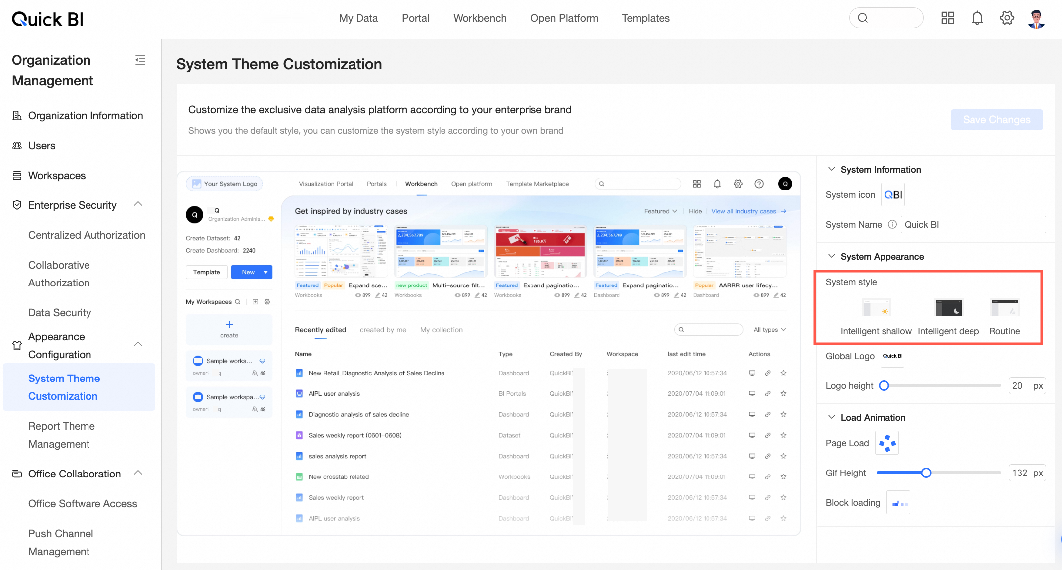
③ Follow system
Follows the system style defined in the custom configuration.
For more information, see Customize the system theme.
NoteOnly organization administrators can set the system style in the custom configuration. The module-level mode setting overrides the organization-level setting.
 icon in the upper-right corner and find the mode switching icon at the bottom to switch between light and dark modes for the workbook.